## Statistical Distribution Plots: Tensor Sample Analysis
### Overview
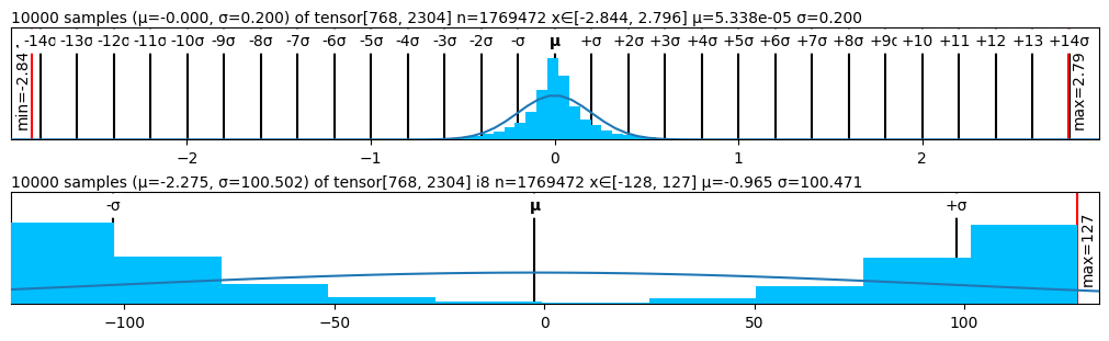
The image displays two vertically stacked statistical plots, each analyzing a sample of 10,000 values drawn from a tensor with shape [768, 2304]. The plots compare the distribution of the raw tensor values (top) against a quantized 8-bit integer representation (i8) of the same data (bottom). Both plots include a histogram of the sampled data, statistical annotations, and a fitted distribution curve.
### Components/Axes
**Top Plot:**
* **Title:** `10000 samples (μ=-0.000, σ=0.200) of tensor[768, 2304] n=1769472 x∈[-2.844, 2.796] μ=5.338e-05 σ=0.200`
* **X-Axis:**
* **Primary Scale:** Numerical values from approximately -2.5 to 2.5, with major ticks at -2, -1, 0, 1, 2.
* **Secondary Scale (Top):** Standard deviation markers from `-14σ` to `+14σ`, centered on `μ`.
* **Range Annotations:** `min=-2.84` (left, vertical red line), `max=2.796` (right, vertical red line).
* **Y-Axis:** Represents frequency/count (no explicit label). The scale is linear.
* **Data Series:** A blue histogram representing the sampled data distribution.
* **Overlay:** A smooth, light blue curve representing a fitted normal (Gaussian) distribution.
* **Statistical Markers:** A vertical black line at the mean (`μ`), and vertical lines at `-σ` and `+σ`.
**Bottom Plot:**
* **Title:** `10000 samples (μ=-2.275, σ=100.502) of tensor[768, 2304] i8 n=1769472 x∈[-128, 127] μ=-0.965 σ=100.471`
* **X-Axis:**
* **Scale:** Numerical values from -128 to 127, with major ticks at -100, -50, 0, 50, 100.
* **Range Annotations:** `min=-128` (implied by axis start), `max=127` (right, vertical red line).
* **Y-Axis:** Represents frequency/count (no explicit label). The scale is linear.
* **Data Series:** A blue histogram representing the sampled data distribution for the i8 quantized values.
* **Overlay:** A straight, light blue line with a slight positive slope, representing a linear fit to the histogram.
* **Statistical Markers:** A vertical black line at the mean (`μ`), and vertical lines at `-σ` and `+σ`.
### Detailed Analysis
**Top Plot (Raw Tensor Values):**
* **Distribution Shape:** The histogram forms a classic, symmetric bell curve centered at zero.
* **Trend Verification:** The data series (blue bars) follows the overlaid normal distribution curve (light blue line) almost perfectly, indicating the raw tensor values are normally distributed.
* **Key Data Points:**
* Sample Mean (μ): 5.338e-05 (effectively 0).
* Sample Standard Deviation (σ): 0.200.
* Theoretical Distribution Parameters (from title): μ=-0.000, σ=0.200.
* Full Data Range: [-2.844, 2.796].
* The histogram's peak is at x=0. The vast majority of data lies within ±1σ (±0.2), with very thin tails extending to ±3σ and beyond.
**Bottom Plot (i8 Quantized Values):**
* **Distribution Shape:** The histogram is bimodal and heavily skewed, with large concentrations of values at the extreme ends of the range (-128 and 127) and very few values in the center.
* **Trend Verification:** The data series (blue bars) does **not** follow the overlaid linear fit (light blue line). The linear line is a poor representation of the actual bimodal distribution.
* **Key Data Points:**
* Sample Mean (μ): -0.965.
* Sample Standard Deviation (σ): 100.471.
* Theoretical Distribution Parameters (from title): μ=-2.275, σ=100.502.
* Full Data Range: [-128, 127] (the full range of an 8-bit signed integer).
* The highest frequency bars are at the minimum (-128) and maximum (127) values. There is a smaller, secondary cluster of values between approximately -75 and -50.
### Key Observations
1. **Radical Distribution Change:** The process of quantizing the normally distributed raw tensor values (top) to the i8 integer range (bottom) completely transforms the distribution from a unimodal Gaussian to a bimodal, extreme-heavy distribution.
2. **Saturation Clipping:** The i8 plot shows clear evidence of saturation clipping. Values from the original normal distribution that fell outside the [-128, 127] range were clamped to these boundaries, creating the large spikes at the ends.
3. **Mean Shift:** The mean shifts from ~0 in the raw data to -0.965 in the i8 data, indicating a slight negative bias introduced by the quantization process.
4. **Variance Explosion:** The standard deviation increases dramatically from 0.200 to 100.471, which is expected as the data is stretched across a much larger numerical range (from a span of ~5.6 to a span of 255).
5. **Poor Linear Fit:** The linear fit applied to the i8 histogram is inappropriate and misleading for this bimodal data.
### Interpretation
This visualization demonstrates the profound impact of **quantization** on data distribution, a critical concept in model compression and deployment.
* **What it shows:** The top plot likely represents the distribution of weights or activations in a neural network layer (e.g., in a transformer model, given the tensor shape [768, 2304]). These values are typically initialized or trained to follow a normal distribution around zero. The bottom plot shows the result of converting these floating-point values to the 8-bit integer format (i8) used for efficient computation on specialized hardware.
* **Why it matters:** The bimodal distribution in the i8 plot is a classic signature of **naive or poorly calibrated quantization**. It indicates that the original data's dynamic range (centered at 0 with σ=0.2) was much narrower than the target i8 range [-128, 127]. Simply mapping the floating-point range to the integer range without proper scaling (e.g., using a scale factor and zero-point) causes most values to be pushed to the extremes, losing almost all nuanced information in the middle. This can severely degrade model accuracy.
* **Underlying Message:** The image serves as a technical diagnostic. It argues for the necessity of **advanced quantization techniques** (like quantization-aware training or calibration) that preserve the shape of the original distribution by appropriately scaling it into the integer range, rather than just clipping it. The poor linear fit further emphasizes that the resulting data structure is complex and not easily summarized by simple statistics.