# Technical Data Extraction: Conductance vs. Twisting Angle in Transition Metal Dichalcogenides
This document provides a comprehensive extraction of data from a series of four scientific plots showing the relationship between conductance ($G$) and twisting angle ($\theta$) for different materials at a fixed Fermi energy ($E_F = +0.5$ meV).
## 1. General Metadata
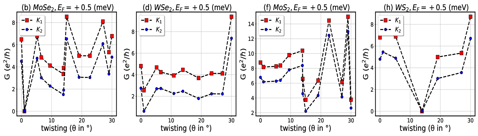
* **Image Type:** Multi-panel line graph (4 panels).
* **Y-Axis Label (All Panels):** $G$ ($e^2/h$) - Conductance in units of the conductance quantum.
* **X-Axis Label (All Panels):** twisting ($\theta$ in $^\circ$) - Twisting angle in degrees.
* **X-Axis Range:** $0^\circ$ to $30^\circ$.
* **Legend (All Panels):**
* **Red Squares (dashed line):** $K_1$
* **Blue Circles (dashed line):** $K_2$
* **Legend Location:** Top-left of each plot area.
* **Common Features:** All plots show a highly oscillatory behavior with $K_1$ consistently maintaining higher conductance values than $K_2$ across most angles.
---
## 2. Panel (b): $MoSe_2, E_F = +0.5$ (meV)
### Trend Analysis
* **$K_1$ (Red):** Starts high (~6.5), drops sharply to 0 at $\theta \approx 1^\circ$, then exhibits a "W" shaped oscillation between $5^\circ$ and $15^\circ$, peaking near 8.5 at $15^\circ$. It stabilizes around 5.0 between $20^\circ-25^\circ$ before a final peak at $28^\circ$.
* **$K_2$ (Blue):** Follows a similar oscillatory pattern but at a lower magnitude. It also hits 0 at $\theta \approx 1^\circ$.
### Data Points (Approximate)
| Twisting $\theta$ ($^\circ$) | $K_1$ Conductance ($e^2/h$) | $K_2$ Conductance ($e^2/h$) |
| :--- | :--- | :--- |
| 0 | 6.5 | 4.5 |
| 1 | 0.0 | 0.0 |
| 5 | 6.8 | 4.8 |
| 7 | 4.9 | 3.0 |
| 14 | 3.3 | 1.5 |
| 15 | 8.5 | 6.5 |
| 19 | 5.0 | 3.1 |
| 23 | 5.0 | 3.1 |
| 27 | 8.1 | 6.1 |
| 29 | 5.4 | 3.4 |
| 30 | 6.8 | 4.9 |
---
## 3. Panel (d): $WSe_2, E_F = +0.5$ (meV)
### Trend Analysis
* **$K_1$ (Red):** Relatively stable compared to other panels. It fluctuates between 4.0 and 5.0 for most of the range before a sharp spike to ~9.5 at $30^\circ$.
* **$K_2$ (Blue):** Shows a significant dip to near 0 at $\theta \approx 1^\circ$, then remains consistently lower than $K_1$ (between 2.0 and 3.0) until a sharp rise to ~7.5 at $30^\circ$.
### Data Points (Approximate)
| Twisting $\theta$ ($^\circ$) | $K_1$ Conductance ($e^2/h$) | $K_2$ Conductance ($e^2/h$) |
| :--- | :--- | :--- |
| 0 | 4.8 | 2.8 |
| 1 | 2.6 | 0.6 |
| 5 | 4.7 | 2.7 |
| 7 | 4.3 | 2.7 |
| 11 | 4.0 | 2.3 |
| 14 | 4.5 | 2.5 |
| 19 | 3.7 | 1.8 |
| 23 | 4.1 | 2.2 |
| 27 | 4.2 | 2.2 |
| 30 | 9.5 | 7.4 |
---
## 4. Panel (f): $MoS_2, E_F = +0.5$ (meV)
### Trend Analysis
* **$K_1$ (Red):** Shows a gradual upward trend from $0^\circ$ to $14^\circ$, followed by a sharp drop to ~4.0 at $15^\circ$. It then recovers with a massive peak of ~14.5 at $23^\circ$ and another peak at $29^\circ$.
* **$K_2$ (Blue):** Mirrors the $K_1$ trend closely but shifted down by approximately 2 units. It reaches its lowest point (~2.2) at $15^\circ$.
### Data Points (Approximate)
| Twisting $\theta$ ($^\circ$) | $K_1$ Conductance ($e^2/h$) | $K_2$ Conductance ($e^2/h$) |
| :--- | :--- | :--- |
| 0 | 8.8 | 6.8 |
| 1 | 8.2 | 6.2 |
| 5 | 8.3 | 6.3 |
| 7 | 8.4 | 6.4 |
| 10 | 9.8 | 7.8 |
| 14 | 10.4 | 8.4 |
| 15 | 3.8 | 2.2 |
| 19 | 6.4 | 4.3 |
| 23 | 14.5 | 12.5 |
| 27 | 6.1 | 4.2 |
| 29 | 15.0 | 13.0 |
| 30 | 3.8 | 2.7 |
---
## 5. Panel (h): $WS_2, E_F = +0.5$ (meV)
### Trend Analysis
* **$K_1$ (Red):** Starts at ~6.8, maintains this until $5^\circ$, then drops linearly to 0 at $\theta \approx 14^\circ$. It then recovers steadily, ending at a peak of ~8.8 at $30^\circ$.
* **$K_2$ (Blue):** Follows the same "V" shape as $K_1$. It starts lower (~4.8), hits 0 at $14^\circ$, and ends at ~6.8 at $30^\circ$.
### Data Points (Approximate)
| Twisting $\theta$ ($^\circ$) | $K_1$ Conductance ($e^2/h$) | $K_2$ Conductance ($e^2/h$) |
| :--- | :--- | :--- |
| 0 | 6.8 | 4.8 |
| 1 | 6.8 | 5.4 |
| 5 | 6.8 | 4.9 |
| 14 | 0.0 | 0.0 |
| 19 | 5.0 | 3.0 |
| 27 | 5.4 | 3.5 |
| 30 | 8.8 | 6.8 |