\n
## Line Chart: Per-Period Regret vs. Time Period
### Overview
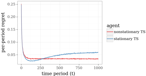
This image presents a line chart illustrating the per-period regret of two agents – one operating in a stationary time series (TS) environment and another in a nonstationary TS environment – over a time period of 1000 units. The chart aims to compare the performance of the agents in terms of regret accumulation.
### Components/Axes
* **X-axis:** "time period (t)", ranging from approximately 0 to 1000. The axis is linearly scaled.
* **Y-axis:** "per-period regret", ranging from approximately 0 to 0.25. The axis is linearly scaled.
* **Legend:** Located in the top-right corner, identifying the two data series:
* "nonstationary TS" (represented by a red line)
* "stationary TS" (represented by a blue line)
* **Gridlines:** A light gray grid is present to aid in reading values.
### Detailed Analysis
The chart displays two lines representing the per-period regret over time.
* **Nonstationary TS (Red Line):** The line starts at approximately 0.045 at t=0, rapidly decreases to a minimum of approximately 0.03 at t=100, and then fluctuates around 0.035-0.04 for the remainder of the time period, ending at approximately 0.036 at t=1000. The line exhibits a generally flat trend after the initial decrease.
* **Stationary TS (Blue Line):** The line begins at approximately 0.05 at t=0, decreases to a minimum of approximately 0.04 at t=100, and then gradually increases to approximately 0.055 by t=1000. The line shows a slight upward trend after the initial decrease.
### Key Observations
* Both agents experience a decrease in per-period regret initially.
* The nonstationary TS agent maintains a lower per-period regret throughout the entire time period compared to the stationary TS agent.
* The stationary TS agent's per-period regret shows a slight increasing trend over time, while the nonstationary TS agent's regret remains relatively stable after the initial decrease.
* The difference in per-period regret between the two agents becomes more pronounced as time progresses.
### Interpretation
The data suggests that the agent operating in a nonstationary time series environment exhibits better performance in terms of regret minimization compared to the agent in a stationary environment. The initial decrease in regret for both agents likely represents a learning phase where the agents adapt to their respective environments. The subsequent stabilization of regret for the nonstationary agent indicates that it has effectively adapted to the changing dynamics of its environment. The slight increase in regret for the stationary agent could be due to the inherent limitations of its learning algorithm in a static environment, or potentially due to noise or random fluctuations. The difference in performance highlights the importance of adapting to nonstationary environments in reinforcement learning or decision-making tasks. The chart demonstrates that an agent capable of handling non-stationarity can achieve lower long-term regret.