## Chart: Probability Distribution of q for Different l Values
### Overview
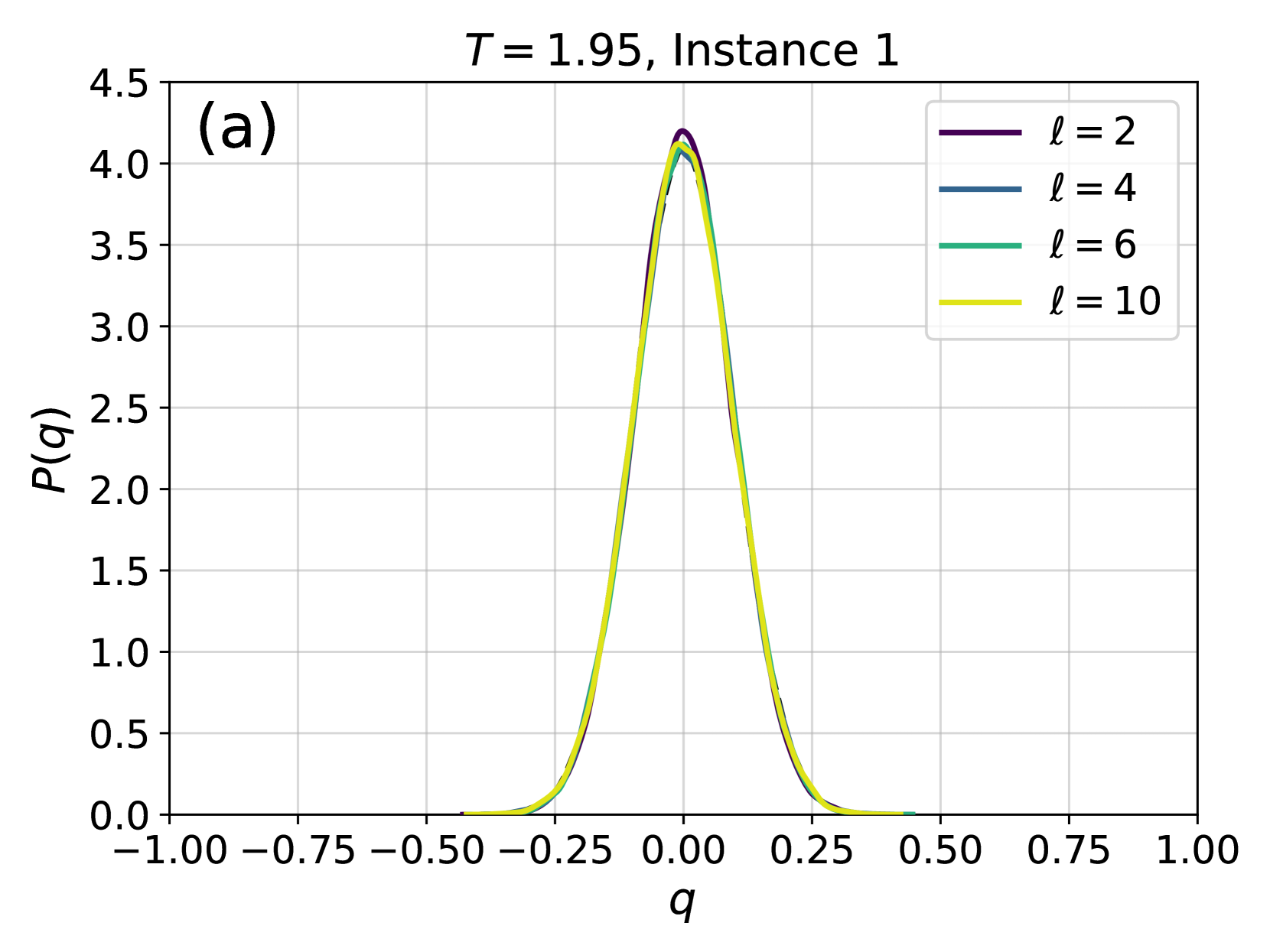
The image presents a line chart illustrating the probability distribution of a variable 'q' for different values of 'l'. The chart is labeled with "T = 1.95, Instance 1" indicating specific parameters for the data. The y-axis represents the probability P(q), and the x-axis represents the variable q. Four different lines are plotted, each corresponding to a different value of 'l' (2, 4, 6, and 10).
### Components/Axes
* **Title:** T = 1.95, Instance 1 (top-center)
* **X-axis Label:** q (bottom-center)
* Scale: -1.00 to 1.00, with markers at -0.75, -0.50, -0.25, 0.00, 0.25, 0.50, 0.75, 1.00
* **Y-axis Label:** P(q) (left-center)
* Scale: 0.0 to 4.5, with markers at 0.0, 0.5, 1.0, 1.5, 2.0, 2.5, 3.0, 3.5, 4.0, 4.5
* **Legend:** Located in the top-right corner.
* l = 2 (Purple)
* l = 4 (Blue)
* l = 6 (Green)
* l = 10 (Yellow)
### Detailed Analysis
The chart displays four probability distributions.
* **l = 2 (Purple):** The line starts at approximately P(q) = 0.0 at q = -1.00. It rises to a peak at approximately q = 0.0, reaching a maximum P(q) of approximately 4.1. It then declines back to approximately P(q) = 0.0 at q = 1.00. The distribution is relatively narrow and symmetrical around q = 0.
* **l = 4 (Blue):** This line also starts at approximately P(q) = 0.0 at q = -1.00. It rises to a peak at approximately q = 0.0, reaching a maximum P(q) of approximately 4.0. It then declines back to approximately P(q) = 0.0 at q = 1.00. This distribution is also narrow and symmetrical, but slightly broader than the l = 2 distribution.
* **l = 6 (Green):** Similar to the previous lines, it starts at approximately P(q) = 0.0 at q = -1.00. It peaks at approximately q = 0.0, reaching a maximum P(q) of approximately 3.8. It declines back to approximately P(q) = 0.0 at q = 1.00. This distribution is broader than the l = 4 distribution.
* **l = 10 (Yellow):** This line starts at approximately P(q) = 0.0 at q = -1.00. It peaks at approximately q = 0.0, reaching a maximum P(q) of approximately 3.5. It declines back to approximately P(q) = 0.0 at q = 1.00. This distribution is the broadest of the four.
All four lines exhibit a bell-shaped curve, characteristic of a probability distribution. The peak of each curve is located at q = 0.0.
### Key Observations
* As 'l' increases, the peak of the probability distribution decreases.
* As 'l' increases, the width of the probability distribution increases.
* All distributions are symmetrical around q = 0.0.
* The distributions are centered around q = 0.
### Interpretation
The chart demonstrates how the probability distribution of 'q' changes as the parameter 'l' varies, while keeping 'T' constant at 1.95. The decreasing peak height and increasing width of the distributions as 'l' increases suggest that as 'l' grows, the values of 'q' become more dispersed and less concentrated around the central value of 0. This could indicate increasing uncertainty or variability in 'q' as 'l' increases. The parameter 'T' likely represents a temperature or a scaling factor, and the instance number suggests this is one realization of a stochastic process. The relationship between 'l' and the distribution of 'q' could be related to a statistical model where 'l' controls the degrees of freedom or the precision of the distribution. The distributions are likely normalized, as the area under each curve represents the total probability, which is equal to 1.