## Line Chart: Dual Distribution Comparison
### Overview
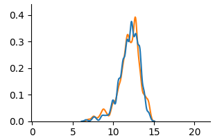
The image displays a 2D line chart comparing two data series (blue and orange lines) plotted against a common x-axis. The chart appears to show two probability distributions or frequency curves that are highly similar in shape and location, with both peaking in the same region. There is no chart title, axis titles, or legend present.
### Components/Axes
* **X-Axis:** A horizontal numerical axis ranging from 0 to 20. Major tick marks and labels are present at intervals of 5 (0, 5, 10, 15, 20).
* **Y-Axis:** A vertical numerical axis ranging from 0.0 to 0.4. Major tick marks and labels are present at intervals of 0.1 (0.0, 0.1, 0.2, 0.3, 0.4).
* **Data Series:**
* **Blue Line:** A continuous, relatively smooth line.
* **Orange Line:** A continuous line with more visible local fluctuations or noise compared to the blue line.
* **Legend:** **Not present.** The meaning of the blue and orange lines is not defined within the image.
* **Titles:** **Not present.** There is no main chart title, x-axis title, or y-axis title.
### Detailed Analysis
**Spatial Grounding & Trend Verification:**
1. **Blue Line Trend:** The line begins near y=0 at approximately x=6. It slopes upward, becoming steeper after x=10, and reaches its primary peak in the region of x=12 to x=13. The peak value is approximately y=0.38. After the peak, it slopes downward sharply, returning to near y=0 by x=15.
2. **Orange Line Trend:** The line follows a very similar path to the blue line. It also begins near y=0 around x=6, slopes upward, and peaks in the same x=12 to x=13 region. Its peak appears slightly higher and sharper than the blue line's peak, reaching approximately y=0.40. It then descends sharply, also reaching near y=0 by x=15.
3. **Key Data Points (Approximate):**
* **Onset (y > 0):** Both lines begin to rise from the baseline at x ≈ 6.
* **Primary Peak Region (x ≈ 12-13):**
* Blue Line Peak: ~ (x=12.5, y=0.38)
* Orange Line Peak: ~ (x=12.8, y=0.40)
* **Secondary Features:** The orange line shows a minor local peak or shoulder around x=11 (y≈0.32) and more jaggedness on the ascending slope between x=8 and x=11. The blue line is smoother in this region.
* **Termination:** Both lines return to the baseline (y ≈ 0) at x ≈ 15.
### Key Observations
1. **High Similarity:** The two distributions are nearly identical in their overall location (centered near x=12.5) and spread (spanning from x≈6 to x≈15).
2. **Noise/Variance Difference:** The primary visual difference is the smoothness of the curves. The orange line exhibits more high-frequency variation, suggesting it may represent noisier data, a different sampling method, or a model with less smoothing compared to the blue line.
3. **Peak Discrepancy:** The orange line's peak is slightly higher and occurs at a marginally higher x-value than the blue line's peak.
4. **Missing Context:** The complete absence of labels, titles, and a legend makes it impossible to determine what these distributions represent (e.g., signal strength, error rates, population data, model predictions).
### Interpretation
The chart demonstrates two datasets or models that produce remarkably similar output distributions. The core phenomenon they measure is concentrated in the range of x=10 to x=14, with a mode near x=12.5.
* **What the data suggests:** The strong overlap implies that whatever underlying process or signal is being captured, both the blue and orange series are detecting it with high fidelity. The difference in smoothness is the most salient point of divergence. This could indicate:
* **Blue:** A smoothed average, a theoretical model, or data from a less noisy sensor.
* **Orange:** Raw experimental data, a model with stochastic elements, or data from a noisier measurement process.
* **Why it matters:** Without labels, the practical significance is unknown. However, in a technical context, this comparison would be critical for validating a new measurement technique (orange) against a established standard (blue), or for comparing the output of a noisy simulation (orange) to a clean analytical solution (blue). The close match would generally be a positive result, indicating good agreement, while the noise characteristic would be a key factor for further analysis.
* **Notable Anomaly:** The most significant "anomaly" is the lack of metadata. For a technical document, this chart is incomplete. The information required to interpret it—axis definitions, series labels, and a title—is entirely absent from the visual itself.