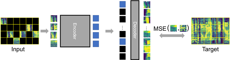
## Diagram: Autoencoder Architecture with Reconstruction Loss ### Overview The diagram illustrates the flow of data through an autoencoder architecture, demonstrating how input data is compressed, reconstructed, and evaluated for quality. The process includes an encoder, decoder, and mean squared error (MSE) loss function to quantify reconstruction accuracy. ### Components/Axes 1. **Input**: A 4x4 grid of patches with varying color intensities (black, blue, green, yellow). Some patches are fully colored, while others are partially filled or empty. 2. **Encoder**: A gray rectangular block labeled "Encoder," representing the dimensionality reduction phase. It processes the input into a compressed representation (blue squares). 3. **Decoder**: A gray rectangular block labeled "Decoder," responsible for reconstructing the input from the compressed representation. It outputs a grid of patches similar to the input. 4. **Target**: A 4x4 grid of patches with distinct color distributions compared to the input, serving as the ground truth for reconstruction. 5. **MSE (Mean Squared Error)**: A bidirectional arrow labeled "MSE" connecting the decoder output to the target, indicating the loss function used to optimize the model. ### Detailed Analysis - **Input**: The input grid contains 16 patches. Approximately 6 patches are fully colored (mix of blue, green, yellow), 4 patches are partially filled, and 6 patches are empty (black). The spatial arrangement suggests localized features. - **Encoder**: Converts the input into a compressed representation (blue squares). The exact dimensions of the compressed representation are not specified but are implied to be smaller than the input. - **Decoder**: Expands the compressed representation back into a grid format. The decoder output matches the input's 4x4 structure but with altered patch distributions. - **Target**: The target grid has 16 patches with a different spatial distribution of colors. Approximately 8 patches are fully colored (predominantly yellow and green), 5 patches are partially filled, and 3 patches are empty. This differs significantly from the input grid. - **MSE**: The bidirectional arrow indicates that the MSE loss is calculated between the decoder's output and the target. This loss drives the optimization of the encoder-decoder parameters to minimize reconstruction error. ### Key Observations 1. **Input vs. Target Discrepancy**: The input and target grids differ in patch distribution, suggesting the autoencoder is trained to reconstruct a target that may not match the original input (e.g., denoising or anomaly detection). 2. **Encoder Compression**: The encoder reduces the input's spatial complexity into a lower-dimensional representation (blue squares), critical for learning efficient features. 3. **Decoder Reconstruction**: The decoder attempts to recover the target structure from the compressed representation, highlighting the model's ability to generalize. 4. **MSE as Optimization Driver**: The MSE loss quantifies the difference between reconstructed and target outputs, guiding the training process to improve accuracy. ### Interpretation This diagram demonstrates the core functionality of an autoencoder: learning a compressed representation of data (via the encoder) and reconstructing it (via the decoder) while minimizing reconstruction error (MSE). The mismatch between input and target implies the model could be used for tasks like: - **Denoising**: Reconstructing clean data from noisy inputs. - **Anomaly Detection**: Identifying inputs where the reconstruction error (MSE) exceeds a threshold. - **Dimensionality Reduction**: Efficiently encoding high-dimensional data into a latent space. The use of MSE as the loss function emphasizes the importance of pixel-level accuracy in reconstruction, which is critical for applications requiring precise output matching (e.g., image restoration). The colored patches likely represent features the model learns to capture, with the encoder-decoder architecture balancing compression and fidelity.