\n
## Heatmap Series: Attention Head Classification by Layer
### Overview
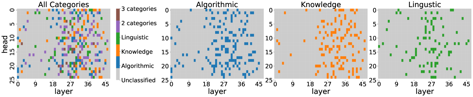
The image displays a series of four horizontally arranged heatmaps. Each heatmap visualizes the classification of attention heads within a neural network model (likely a transformer) across its layers. The first plot shows an aggregate view of all classifications, while the subsequent three plots isolate the distribution for three specific categories: Algorithmic, Knowledge, and Linguistic. The background of all plots is gray, representing unclassified heads.
### Components/Axes
* **Titles (Top of each plot, left to right):** "All Categories", "Algorithmic", "Knowledge", "Linguistic".
* **Y-Axis (Left side of each plot):** Labeled "head". The scale runs from 0 at the top to 25 at the bottom, with major tick marks at 0, 5, 10, 15, 20, and 25. This represents the index of the attention head within a layer.
* **X-Axis (Bottom of each plot):** Labeled "layer". The scale runs from 0 on the left to 45 on the right, with major tick marks at 0, 9, 18, 27, 36, and 45. This represents the layer depth in the model.
* **Legend (Positioned to the right of the "All Categories" plot):**
* **Brown square:** "3 categories"
* **Purple square:** "2 categories"
* **Green square:** "Linguistic"
* **Orange square:** "Knowledge"
* **Blue square:** "Algorithmic"
* **Gray square:** "Unclassified"
### Detailed Analysis
**1. All Categories Plot (Leftmost):**
* **Trend:** This plot shows a composite, overlapping view. Colored squares (representing classified heads) are densely clustered in the central region of the plot.
* **Spatial Distribution:** The highest density of classified heads appears in the range of approximately **layers 18 to 36** and **heads 5 to 20**. Within this cluster, colors are heavily intermixed, indicating heads classified into multiple categories (brown for 3, purple for 2) or single categories (green, orange, blue).
* **Outliers:** Classified heads are sparse in the early layers (0-9) and the very late layers (36-45), and also in the highest (0-5) and lowest (20-25) head indices.
**2. Algorithmic Plot (Second from left):**
* **Trend:** The blue squares show a scattered but discernible pattern.
* **Spatial Distribution:** Algorithmic heads are most concentrated in the **mid-to-late layers**, roughly **layers 18 to 36**. They are distributed across a wide range of head indices within those layers, with a slight concentration in the middle head indices (5-20). Very few are present before layer 9 or after layer 40.
**3. Knowledge Plot (Third from left):**
* **Trend:** The orange squares form a distinct, dense cluster.
* **Spatial Distribution:** Knowledge heads are highly concentrated in the **later layers**, primarily between **layers 27 and 45**. Their head index distribution is broad but densest between **heads 5 and 20**. This category shows the clearest localization to a specific layer range.
**4. Linguistic Plot (Rightmost):**
* **Trend:** The green squares are the most widely dispersed of the three isolated categories.
* **Spatial Distribution:** Linguistic heads are found across a broad swath of the model, from approximately **layer 9 to layer 36**. They are not confined to a tight layer band like Knowledge. Their distribution across head indices is also relatively even within the active layer range, though slightly sparser at the very top (head 0) and bottom (head 25).
### Key Observations
1. **Layer Specialization:** There is a clear progression of functional specialization along the layer axis. Linguistic processing appears earlier and is more distributed, Algorithmic processing peaks in the middle layers, and Knowledge processing is strongly concentrated in the final third of the model.
2. **Head Multiplexing:** The presence of brown ("3 categories") and purple ("2 categories") squares in the "All Categories" plot confirms that individual attention heads can be involved in multiple types of processing simultaneously.
3. **Unclassified Majority:** The dominant gray background across all plots indicates that the majority of attention heads (across all layers and indices) were not classified into any of the three specified categories by the analysis method used.
4. **Spatial Overlap:** The dense cluster in the "All Categories" plot corresponds to the region where the Algorithmic, Knowledge, and Linguistic distributions overlap, particularly in layers 18-36.
### Interpretation
This visualization provides a functional map of a large language model's internal processing. It suggests a hierarchical or staged processing flow:
* **Early-to-Mid Layers (Linguistic Foundation):** Linguistic processing is distributed across a wide range of layers, forming a foundational capability that is likely engaged throughout processing.
* **Mid Layers (Algorithmic Processing):** A more specialized set of heads in the central layers appears dedicated to algorithmic or procedural tasks, such as syntactic parsing, logical reasoning, or step-by-step computation.
* **Late Layers (Knowledge Retrieval/Application):** The final layers are heavily specialized for accessing and applying factual or world knowledge, likely integrating the processed linguistic and algorithmic information to generate informed outputs.
The concentration of multi-category heads in the central overlap zone suggests this is a critical integration region where linguistic structure, reasoning algorithms, and factual knowledge converge. The high proportion of unclassified heads implies either that the classification scheme is not exhaustive, or that many heads perform functions not captured by these three categories (e.g., coreference, sentiment, stylistic control). This map is crucial for understanding model interpretability, identifying potential points for intervention or pruning, and guiding architectural design.