## Chart: Success Probability and Iteration-to-Solution vs. Problem Size
### Overview
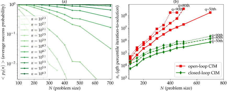
The image presents two plots side-by-side, labeled (a) and (b). Plot (a) shows the average success probability as a function of problem size for different values of 'n'. Plot (b) shows the qth percentile iteration-to-solution as a function of problem size for open-loop and closed-loop CIM.
### Components/Axes
**Plot (a):**
* **Title:** (a)
* **X-axis:** N (problem size), linear scale from 100 to 700 in increments of 100.
* **Y-axis:** <p₀(n)> (average success probability), logarithmic scale from 10⁻² to 10⁰.
* **Legend:** Located on the left side of the plot. Each line represents a different value of 'n':
* Lightest Green: n = 10²·³
* n = 10²·⁷
* n = 10³·¹
* n = 10³·⁵
* n = 10³·⁹
* n = 10⁴·³
* n = 10⁴·⁷
* n = 10⁵·¹
* n = 10⁵·⁵
* n = 10⁵·⁹
* Darkest Green: n = 10⁶·³
**Plot (b):**
* **Title:** (b)
* **X-axis:** N (problem size), linear scale from 0 to 800 in increments of 200.
* **Y-axis:** nₛ (qth percentile iteration-to-solution), logarithmic scale from 10³ to 10⁸.
* **Legend:** Located at the bottom of the plot.
* Red squares: open-loop CIM
* Green diamonds: closed-loop CIM
* **Percentiles:** q = 50th, 80th, 90th are marked for both open-loop and closed-loop CIM.
### Detailed Analysis
**Plot (a): Average Success Probability**
The plot shows the average success probability decreases as the problem size (N) increases. The rate of decrease varies depending on the value of 'n'.
* **n = 10²·³:** The success probability starts near 1 and decreases gradually to approximately 0.01 as N increases from 100 to 700.
* **n = 10²·⁷:** The success probability starts near 1 and decreases gradually to approximately 0.005 as N increases from 100 to 700.
* **n = 10³·¹:** The success probability starts near 1 and decreases gradually to approximately 0.002 as N increases from 100 to 700.
* **n = 10³·⁵:** The success probability starts near 1 and decreases gradually to approximately 0.001 as N increases from 100 to 700.
* **n = 10³·⁹:** The success probability starts near 1 and decreases gradually to approximately 0.0005 as N increases from 100 to 700.
* **n = 10⁴·³:** The success probability starts near 1 and decreases gradually to approximately 0.0002 as N increases from 100 to 700.
* **n = 10⁴·⁷:** The success probability starts near 1 and decreases gradually to approximately 0.0001 as N increases from 100 to 700.
* **n = 10⁵·¹:** The success probability starts near 1 and decreases gradually to approximately 0.00005 as N increases from 100 to 700.
* **n = 10⁵·⁵:** The success probability starts near 1 and decreases gradually to approximately 0.00002 as N increases from 100 to 700.
* **n = 10⁵·⁹:** The success probability starts near 1 and decreases gradually to approximately 0.00001 as N increases from 100 to 700.
* **n = 10⁶·³:** The success probability remains close to 1 across the entire range of N values.
**Plot (b): Qth Percentile Iteration-to-Solution**
The plot shows the qth percentile iteration-to-solution increases as the problem size (N) increases. Open-loop CIM generally requires more iterations than closed-loop CIM for the same problem size and percentile.
* **Open-loop CIM (Red):**
* q = 50th (solid line): Increases from approximately 10⁴ at N=100 to approximately 2 * 10⁶ at N=700.
* q = 80th (dashed line): Increases from approximately 2 * 10⁴ at N=100 to approximately 6 * 10⁶ at N=500.
* q = 90th (dotted line): Increases from approximately 3 * 10⁴ at N=100 to approximately 10⁷ at N=500.
* **Closed-loop CIM (Green):**
* q = 50th (solid line): Increases from approximately 10⁴ at N=100 to approximately 2 * 10⁵ at N=700.
* q = 80th (dashed line): Increases from approximately 2 * 10⁴ at N=100 to approximately 3 * 10⁵ at N=500.
* q = 90th (dotted line): Increases from approximately 3 * 10⁴ at N=100 to approximately 4 * 10⁵ at N=500.
### Key Observations
* In plot (a), as 'n' increases, the average success probability becomes less sensitive to changes in problem size (N).
* In plot (b), the number of iterations required to reach a solution increases with problem size for both open-loop and closed-loop CIM.
* Open-loop CIM generally requires significantly more iterations than closed-loop CIM to reach a solution.
* Higher percentiles (q = 80th, 90th) require more iterations than lower percentiles (q = 50th).
### Interpretation
The plots demonstrate the trade-offs between success probability and the number of iterations required to solve a problem using different CIM approaches. Plot (a) shows that for larger values of 'n', the success probability remains high even for larger problem sizes. However, plot (b) shows that closed-loop CIM generally requires fewer iterations to reach a solution compared to open-loop CIM, suggesting it is more efficient. The choice between open-loop and closed-loop CIM, and the selection of 'n', would depend on the specific requirements of the problem, balancing the need for high success probability with the desire for efficient computation.