## Diagram: Reservoir Computing Network ### Overview The image is a diagram illustrating the architecture of a reservoir computing network. It consists of three main layers: an input layer, a dynamic reservoir layer, and an output layer. The diagram shows the connections between these layers and highlights the fixed and trainable weights within the network. ### Components/Axes * **Input Layer:** Located on the left side of the diagram. Contains a series of purple nodes. Labeled "Input layer" at the top and "Input x(t)" at the bottom. * **Dynamic Reservoir Layer:** Located in the center of the diagram. Contains a network of interconnected orange nodes within a shaded orange region. Labeled "Dynamic reservoir layer" at the top and "Internal states r(t)" at the bottom. * **Output Layer:** Located on the right side of the diagram. Contains a series of teal nodes. Labeled "Output layer" at the top and "Output y(t)" at the bottom. * **Connections:** Arrows indicate the flow of information between the layers. Connections from the input layer to the reservoir layer and from the reservoir layer to the output layer. The reservoir layer also contains internal connections. * **Weights:** The connections between the input layer and the reservoir layer are labeled as "Fixed". The connections between the reservoir layer and the output layer are labeled as "Trainable weights". ### Detailed Analysis * **Input Layer:** The input layer consists of at least 3 purple nodes, with an ellipsis indicating that there may be more. Each node in the input layer has connections to multiple nodes in the dynamic reservoir layer. * **Dynamic Reservoir Layer:** The dynamic reservoir layer is the core of the network. It consists of approximately 10 orange nodes interconnected in a complex, recurrent manner. The connections within the reservoir are represented by curved arrows, indicating feedback loops. The entire reservoir is contained within a shaded orange region. * **Output Layer:** The output layer consists of at least 3 teal nodes, with an ellipsis indicating that there may be more. Each node in the output layer receives input from multiple nodes in the dynamic reservoir layer. * **Connections:** The connections between the input layer and the reservoir layer appear to be randomly distributed. The connections between the reservoir layer and the output layer are also distributed. * **Weights:** The diagram explicitly labels the weights between the input and reservoir layers as "Fixed," implying that these connections are not adjusted during training. The weights between the reservoir and output layers are labeled as "Trainable weights," indicating that these connections are adjusted during the training process. ### Key Observations * The dynamic reservoir layer is a complex, recurrent network. * The connections between the input layer and the reservoir layer are fixed. * The connections between the reservoir layer and the output layer are trainable. ### Interpretation The diagram illustrates the fundamental architecture of a reservoir computing network. The key idea behind reservoir computing is to use a fixed, randomly connected recurrent neural network (the dynamic reservoir layer) to map the input signal into a higher-dimensional space. The output layer is then trained to read out the desired output from this high-dimensional representation. The fixed weights between the input and reservoir layers allow the reservoir to act as a non-linear feature extractor. The trainable weights between the reservoir and output layers allow the network to learn the mapping from the reservoir's internal states to the desired output. The recurrent connections within the reservoir allow the network to process temporal data, making it suitable for tasks such as speech recognition, time series prediction, and control. The complexity of the reservoir's internal connections is crucial for its ability to capture the dynamics of the input signal.

\n ## Diagram: Echo State Network (Reservoir Computing) Architecture ### Overview The image depicts the architecture of an Echo State Network (ESN), a type of recurrent neural network (RNN) that falls under the broader category of reservoir computing. The diagram illustrates the three main layers: an input layer, a dynamic reservoir layer, and an output layer. The connections between these layers are shown, highlighting the fixed input weights and trainable output weights. ### Components/Axes The diagram consists of three main sections: * **Input Layer:** Located on the left side, represented by purple circles. Labeled "Input layer" and "Input x(t)". * **Dynamic Reservoir Layer:** Occupies the central portion of the diagram, depicted as a light yellow, amorphous shape containing orange circles. Labeled "Dynamic reservoir layer" and "Internal states r(t)". * **Output Layer:** Situated on the right side, represented by teal circles. Labeled "Output layer" and "Output y(t)". * **Fixed Weights:** Indicated by lines connecting the input layer to the reservoir layer. Labeled "Fixed". * **Trainable Weights:** Indicated by lines connecting the reservoir layer to the output layer. Labeled "Trainable weights". * **Connections within Reservoir:** Numerous curved lines connect the orange circles within the reservoir layer, representing recurrent connections. * **Ellipsis:** Three dots are present in the input and output layers, indicating that the layers can have more nodes than are explicitly shown. ### Detailed Analysis / Content Details The diagram shows a fully connected input layer feeding into the dynamic reservoir layer. The reservoir layer consists of approximately 10 orange circles, interconnected by numerous connections. The connections within the reservoir are not explicitly weighted or labeled. The reservoir layer then connects to the output layer, which consists of approximately 5 teal circles. * **Input Layer:** Contains at least 4 nodes (plus ellipsis indicating more). * **Reservoir Layer:** Contains approximately 10 nodes. The connections between these nodes are dense and recurrent. * **Output Layer:** Contains at least 4 nodes (plus ellipsis indicating more). * **Input to Reservoir Connections:** Each input node is connected to every node in the reservoir layer. * **Reservoir to Output Connections:** Each reservoir node is connected to every output node. * **Weighting:** The connections from the input layer to the reservoir layer have fixed weights, while the connections from the reservoir layer to the output layer have trainable weights. ### Key Observations The key feature of this architecture is the fixed, randomly generated weights within the reservoir layer. This contrasts with traditional RNNs where all weights are trained. The reservoir layer acts as a non-linear transformation of the input signal, and the output layer learns to extract relevant information from the reservoir's internal states. The diagram emphasizes the recurrent connections within the reservoir, which are crucial for maintaining a "memory" of past inputs. ### Interpretation This diagram illustrates the core concept of reservoir computing, specifically as implemented in an Echo State Network. The reservoir layer, with its fixed random weights and recurrent connections, provides a rich, high-dimensional representation of the input signal. The trainable output weights allow the network to learn to map this representation to the desired output. This approach simplifies training compared to traditional RNNs, as only the output weights need to be adjusted. The diagram highlights the separation of concerns: the reservoir handles the complex non-linear dynamics, while the output layer performs the task-specific learning. The use of fixed weights in the reservoir is a key design choice that enables efficient training and avoids the vanishing/exploding gradient problems often encountered in deep RNNs. The diagram is a conceptual illustration and does not provide specific numerical data or performance metrics. It serves to explain the architecture and the flow of information within the network.

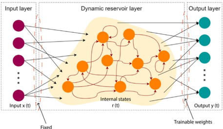
## Diagram: Echo State Network / Reservoir Computing Architecture ### Overview The image is a technical schematic diagram illustrating the architecture of a reservoir computing model, specifically an Echo State Network (ESN). It depicts the flow of information from an input layer, through a complex, recurrently connected "dynamic reservoir" layer, to an output layer. The diagram emphasizes the distinction between fixed and trainable components of the network. ### Components/Axes The diagram is organized into three primary vertical sections, demarcated by dashed gray boxes: 1. **Input layer (Left Section):** * **Visual Elements:** A vertical column of four solid purple circles, with a vertical ellipsis (`...`) below the third circle, indicating additional inputs. * **Labels:** * Top label: `Input layer` * Bottom label: `Input x(t)` * Annotation below the input column: `Fixed` (with an arrow pointing to the connections leaving the input layer). 2. **Dynamic reservoir layer (Center Section):** * **Visual Elements:** A large, irregularly shaped, light-orange cloud containing eight solid orange circles (neurons). These neurons are interconnected by a complex web of red arrows, indicating recurrent connections. Some arrows loop back to the same neuron. * **Labels:** * Top label: `Dynamic reservoir layer` * Label inside the cloud, near the bottom: `Internal states r(t)` 3. **Output layer (Right Section):** * **Visual Elements:** A vertical column of four solid teal circles, with a vertical ellipsis (`...`) below the third circle, indicating additional outputs. * **Labels:** * Top label: `Output layer` * Bottom label: `Output y(t)` * Annotation below the output column: `Trainable weights` (with an arrow pointing to the connections entering the output layer). **Connections and Flow:** * **Input to Reservoir:** Black arrows originate from each purple input neuron and point to multiple orange neurons within the reservoir. The `Fixed` label indicates these input-to-reservoir connection weights are not adjusted during training. * **Reservoir Recurrence:** Red arrows form a dense, recurrent network within the reservoir cloud, connecting orange neurons to each other. * **Reservoir to Output:** Black arrows originate from various orange neurons within the reservoir and point to the teal output neurons. The `Trainable weights` label indicates these reservoir-to-output connection weights are adjusted during training. ### Detailed Analysis * **Spatial Grounding:** The `Fixed` label is positioned at the bottom-left of the diagram, directly associated with the input-to-reservoir connections. The `Trainable weights` label is at the bottom-right, associated with the reservoir-to-output connections. The `Internal states r(t)` label is centered within the reservoir cloud. * **Component Isolation:** * **Header Region:** Contains the three main layer titles. * **Main Diagram Region:** Contains the visual representation of neurons (circles) and connections (arrows) across the three layers. * **Footer Region:** Contains the key annotations `Fixed` and `Trainable weights`. * **Trend/Flow Verification:** The diagram illustrates a clear, unidirectional information flow from left to right: `Input x(t)` → `Dynamic reservoir layer (Internal states r(t))` → `Output y(t)`. The complexity and recurrence are confined to the central reservoir. ### Key Observations 1. **Architectural Dichotomy:** The core design principle highlighted is the separation of the network into a fixed, complex, nonlinear dynamical system (the reservoir) and a simple, trainable linear readout (the output layer). 2. **Recurrent Complexity:** The reservoir is depicted as a "black box" of rich, recurrent dynamics (red arrows), which is the source of the model's computational power for processing temporal sequences. 3. **State Representation:** The label `Internal states r(t)` explicitly identifies the reservoir's activity vector as the dynamic state that is used by the output layer. 4. **Scalability Hint:** The vertical ellipses (`...`) in both the input and output layers indicate that the diagram is a simplified representation and the actual number of input and output dimensions can be larger. ### Interpretation This diagram is a canonical representation of the Echo State Network paradigm within reservoir computing. It visually encodes the core hypothesis of this approach: that a fixed, randomly connected, and nonlinear recurrent neural network (the reservoir) can project input signals into a high-dimensional dynamical space. The temporal patterns within this space (`r(t)`) are then linearly combined by the trainable output weights to produce the desired output `y(t)`. The key takeaway is **efficiency through constraint**. By fixing the vast majority of the network's parameters (the input and internal reservoir connections) and only training the simple output layer, the model avoids the complex, often unstable, training procedures (like backpropagation through time) required for fully trainable recurrent networks. The diagram argues that the "magic" happens in the rich, emergent dynamics of the reservoir, which the output layer merely learns to interpret. The `Fixed` vs. `Trainable` annotation is the most critical piece of information, defining the entire learning philosophy of this architecture.

## Diagram: Reservoir Computing Architecture ### Overview The diagram illustrates a reservoir computing architecture, a type of recurrent neural network (RNN) structure. It consists of three primary components: an input layer, a dynamic reservoir layer, and an output layer. Arrows indicate directional flow and connections between components, with annotations specifying fixed vs. trainable parameters. ### Components/Axes 1. **Input Layer**: - **Nodes**: Purple circles labeled "Input x(t)" (time-dependent input). - **Connections**: Black arrows with red dashed outlines connecting inputs to the reservoir. - **Annotations**: "Fixed" (weights between input and reservoir are static). 2. **Dynamic Reservoir Layer**: - **Nodes**: Orange circles labeled "Internal states r(t)". - **Connections**: Red arrows forming a dense, recurrent network (self-connections and inter-node connections). - **Annotations**: "Internal states" (dynamic, time-dependent processing). 3. **Output Layer**: - **Nodes**: Teal circles labeled "Output y(t)". - **Connections**: Black arrows with red dashed outlines from the reservoir to outputs. - **Annotations**: "Trainable weights" (weights between reservoir and output are optimized during training). 4. **Legend/Annotations**: - **Color Coding**: - Purple: Input layer. - Orange: Reservoir nodes. - Teal: Output layer. - Red: Reservoir internal connections. - Black: Input/output layer connections. - **Key Labels**: - "Fixed" (input-reservoir weights). - "Trainable weights" (reservoir-output weights). ### Detailed Analysis - **Input Layer**: - Receives time-series data `x(t)`. - Fixed weights ensure the input pattern is preserved without modification during training. - **Reservoir Layer**: - Processes inputs through chaotic, high-dimensional dynamics (`r(t)`). - Dense recurrent connections (red arrows) enable complex temporal pattern learning. - No explicit bias terms or activation functions labeled. - **Output Layer**: - Maps reservoir states to desired outputs `y(t)`. - Trainable weights allow the network to learn task-specific mappings from the reservoir's dynamics. ### Key Observations 1. **Fixed vs. Trainable Weights**: - Input-reservoir connections are static ("Fixed"). - Reservoir-output connections are optimized ("Trainable weights"). 2. **Reservoir Dynamics**: - The chaotic, high-connectivity structure suggests a "black box" for feature extraction. - No explicit time-delay elements or gating mechanisms (e.g., LSTM/GRU) are shown. 3. **Output Structure**: - Output nodes are directly connected to reservoir states, implying linear readout (common in reservoir computing). ### Interpretation This architecture demonstrates the core principles of reservoir computing: - **Fixed Input Weights**: Preserve input patterns while allowing the reservoir to learn temporal dynamics. - **Trainable Output Weights**: Enable task-specific learning by adjusting the readout layer. - **Reservoir Complexity**: The dense, recurrent connections create a high-dimensional, chaotic space for feature representation. The diagram emphasizes the separation of timescale learning (reservoir dynamics) and parameter optimization (output weights), a hallmark of reservoir computing's efficiency in handling sequential data. The absence of explicit activation functions or regularization terms suggests a focus on the theoretical framework rather than implementation details.