## 3D Surface Plot: Free Energy vs. θ1 and θ2 ### Overview The image is a 3D surface plot visualizing the relationship between Free Energy and two variables, θ1 and θ2. The surface is colored to represent the magnitude of the Free Energy, with cooler colors (purple/blue) indicating lower energy and warmer colors (yellow/green) indicating higher energy. The plot shows a saddle-like shape, suggesting a minimum along one axis and a maximum along the other. ### Components/Axes * **Vertical Axis (y-axis):** "Free Energy". The scale ranges from approximately -7 to -3. * **Horizontal Axis 1 (x-axis):** "θ2". The scale ranges from -5 to 5. * **Horizontal Axis 2 (z-axis):** "θ1". The scale ranges from -5 to 5. * **Color Scale:** The surface is colored according to the Free Energy value. Purple/blue represents lower values, transitioning to green and yellow for higher values. ### Detailed Analysis The surface plot shows a saddle point. * Along the θ2 axis, the Free Energy initially decreases as θ2 moves away from 0, reaching a minimum around θ2 = ±4. * Along the θ1 axis, the Free Energy increases as θ1 moves away from 0, reaching a maximum around θ1 = ±2. * The lowest Free Energy values (approximately -7) are observed at the corners of the plot where θ1 is near 0 and θ2 is near ±5. * The highest Free Energy values (approximately -3) are observed near the center of the plot where θ1 is near ±2 and θ2 is near 0. ### Key Observations * The plot exhibits a clear saddle point, indicating a minimum energy configuration along one dimension and a maximum along another. * The Free Energy is highly sensitive to changes in both θ1 and θ2. * The global minimum Free Energy is located at the corners of the plot. ### Interpretation The 3D surface plot visualizes the energy landscape of a system with two degrees of freedom, θ1 and θ2. The saddle point suggests that the system has a stable configuration (minimum energy) along one direction (θ2) and an unstable configuration (maximum energy) along another direction (θ1). This type of energy landscape is common in chemical reactions and other physical systems where multiple variables influence the overall energy. The plot provides insights into the stability and dynamics of the system, indicating the preferred configurations and the energy barriers that must be overcome to transition between different states.

\n ## 3D Surface Plot: Free Energy Landscape ### Overview The image depicts a 3D surface plot representing a free energy landscape. The plot visualizes the relationship between two angular parameters, θ₁ and θ₂, and the corresponding free energy. The surface is colored to indicate the free energy value, with warmer colors (yellow/green) representing lower free energy and cooler colors (blue/purple) representing higher free energy. ### Components/Axes * **X-axis:** θ₁ (Theta 1), ranging approximately from -4 to 4. * **Y-axis:** θ₂ (Theta 2), ranging approximately from -4 to 4. * **Z-axis:** Free Energy, ranging approximately from -7 to -3. * **Color Scale:** Represents Free Energy, with a gradient from purple (high energy) to yellow/green (low energy). ### Detailed Analysis The surface exhibits a complex topography with multiple local minima and maxima. * **Main Minimum:** A prominent minimum is located near θ₁ ≈ 0 and θ₂ ≈ 0, with a free energy value of approximately -3. This is indicated by the yellow/green color in that region. * **Secondary Minima:** There are two secondary minima located approximately at: * θ₁ ≈ 3, θ₂ ≈ 2, with a free energy of approximately -4. * θ₁ ≈ -3, θ₂ ≈ -2, with a free energy of approximately -4. * **Saddle Points:** Several saddle points are visible, connecting the minima. These are indicated by regions where the color changes rapidly. * **Maximum:** A maximum is located approximately at θ₁ ≈ -4 and θ₂ ≈ 4, with a free energy of approximately -7. * **Trend:** The surface generally slopes downward from the upper-right to the lower-left, indicating a decreasing free energy in that direction. ### Key Observations * The landscape is not smooth; it has several distinct features. * The primary minimum suggests a stable state at θ₁ ≈ 0 and θ₂ ≈ 0. * The secondary minima suggest metastable states. * The presence of saddle points indicates pathways between different states. ### Interpretation This plot likely represents the free energy landscape of a system with two degrees of freedom, represented by the angles θ₁ and θ₂. The minima on the landscape correspond to stable or metastable states of the system. The height of the energy barriers (represented by the saddle points) determines the rate of transitions between these states. The system will tend to reside in the minimum energy state, but thermal fluctuations can allow it to overcome the energy barriers and explore other states. The shape of the landscape provides insights into the dynamics and stability of the system. The plot suggests that the system has a preferred configuration around θ₁ ≈ 0 and θ₂ ≈ 0, but can also exist in other configurations with slightly higher energy. The complexity of the landscape indicates that the system's behavior may be non-trivial.

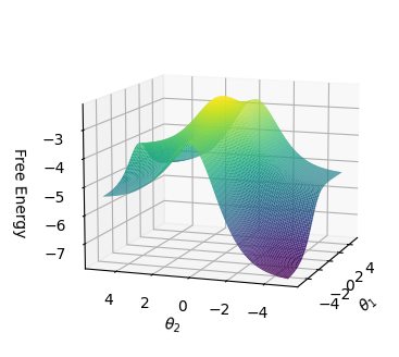
## 3D Surface Plot: Free Energy Landscape ### Overview The image displays a three-dimensional surface plot visualizing a function of two variables, θ₁ and θ₂. The plot illustrates how "Free Energy" varies across a parameter space defined by these two variables. The surface is rendered with a color gradient that maps directly to the Free Energy value, providing an intuitive visual guide to the function's topography. ### Components/Axes * **Vertical Axis (Z-axis):** Labeled **"Free Energy"**. The scale is numerical, with major tick marks at **-3, -4, -5, -6, and -7**. The values are negative, indicating the plotted quantity is likely a negative energy or a log-probability. * **Horizontal Axis 1 (X-axis, front-left):** Labeled **"θ₂"** (theta subscript two). The scale ranges from **-4 to 4**, with major tick marks at **-4, -2, 0, 2, and 4**. * **Horizontal Axis 2 (Y-axis, front-right):** Labeled **"θ₁"** (theta subscript one). The scale also ranges from **-4 to 4**, with major tick marks at **-4, -2, 0, 2, and 4**. * **Surface & Color Mapping:** The plotted surface is a continuous mesh. Its color corresponds to the Free Energy value (Z-axis): * **Yellow/Green:** Represents the highest values of Free Energy (approximately -3 to -4). * **Teal/Blue:** Represents mid-range values (approximately -4 to -6). * **Dark Blue/Purple:** Represents the lowest values of Free Energy (approximately -6 to -7). * **Grid:** A 3D wireframe grid provides spatial reference, with planes corresponding to the major tick marks on all three axes. ### Detailed Analysis * **Spatial Grounding & Trend Verification:** The surface exhibits a single, prominent **peak** (a local and likely global maximum) located near the center of the parameter space, at approximately **(θ₁ ≈ 0, θ₂ ≈ 0)**. At this peak, the Free Energy is at its highest, visually estimated to be **≈ -3.2**. * From this central peak, the surface **slopes downward** in all directions as the absolute values of θ₁ and θ₂ increase. The descent is not perfectly symmetric. * The **lowest points** (global minima) appear to be located near the four corners of the plotted domain, specifically where both |θ₁| and |θ₂| are large (e.g., near (4,4), (4,-4), (-4,4), (-4,-4)). At these corners, the Free Energy reaches its minimum value of **≈ -7.0**. * The surface appears smooth and continuous, with no visible discontinuities, sharp ridges, or secondary peaks within the displayed range. ### Key Observations 1. **Central Maximum:** The most notable feature is the single, smooth peak at the origin (0,0). This suggests the system has a unique state of highest Free Energy when both parameters are zero. 2. **Symmetry:** The landscape shows approximate, but not perfect, symmetry around the θ₁=0 and θ₂=0 planes. The shape resembles a rounded, inverted mountain or a broad hill. 3. **Monotonic Decrease:** Moving away from the origin along any radial direction results in a monotonic decrease in Free Energy. 4. **Color as Value Guide:** The color gradient is a direct and effective visual encoding of the Z-axis value, making the topography immediately interpretable. ### Interpretation This plot likely represents an **energy landscape** or a **negative log-likelihood surface** from a statistical or machine learning model (e.g., a variational autoencoder, a physics-based model, or an optimization problem). * **What it Suggests:** The central peak at (θ₁=0, θ₂=0) represents an **unstable equilibrium point** or a state of maximum "surprise"/energy. The system would naturally tend to move away from this state towards regions of lower Free Energy (the valleys). * **Relationship of Elements:** The two parameters, θ₁ and θ₂, are coupled in defining the system's state. The smooth, convex-like shape around the peak suggests that simple gradient-based optimization methods would efficiently find the minima from most starting points. * **Notable Implications:** The absence of multiple local minima (within this view) implies the optimization problem is relatively simple, with a clear global solution (or set of degenerate solutions at the corners). The landscape's shape is crucial for understanding the dynamics, stability, and learnability of the underlying system. The negative Free Energy values are standard in statistical physics and variational inference, where minimizing Free Energy is equivalent to maximizing a lower bound on model evidence or minimizing an energy function.

## 3D Surface Plot: Free Energy Landscape as a Function of θ₁ and θ₂ ### Overview The image depicts a 3D surface plot representing a free energy landscape with two variables, θ₁ (horizontal axis) and θ₂ (depth axis). The vertical axis represents free energy values ranging from -7 to -3. The surface exhibits a complex topography with multiple peaks, valleys, and saddle points, colored in a gradient from purple (lowest energy) to yellow (highest energy). ### Components/Axes - **Axes Labels**: - **X-axis (θ₁)**: Ranges from -4 to 4 in increments of 2. - **Y-axis (θ₂)**: Ranges from -4 to 4 in increments of 2. - **Z-axis (Free Energy)**: Ranges from -7 to -3 in increments of 1. - **Color Gradient**: - Purple → Yellow: Represents increasing free energy values (no explicit legend, but inferred from color mapping). - **Grid Lines**: Black grid lines define the 3D coordinate system. ### Detailed Analysis 1. **Highest Energy Point**: - **Location**: θ₁ ≈ 0, θ₂ ≈ 0. - **Free Energy**: Approximately -3 (uncertainty: ±0.5). - **Color**: Yellow (consistent with highest energy). 2. **Lowest Energy Point**: - **Location**: θ₁ ≈ -4, θ₂ ≈ -4. - **Free Energy**: Approximately -7 (uncertainty: ±0.5). - **Color**: Purple (consistent with lowest energy). 3. **Saddle Point**: - **Location**: θ₁ ≈ 2, θ₂ ≈ 2. - **Free Energy**: Approximately -4.5 (uncertainty: ±0.5). - **Color**: Green (intermediate energy). 4. **Additional Features**: - **Peaks**: - θ₁ ≈ -2, θ₂ ≈ 2: Free energy ≈ -5 (green). - θ₁ ≈ 2, θ₂ ≈ -2: Free energy ≈ -5 (green). - **Valleys**: - θ₁ ≈ -3, θ₂ ≈ 3: Free energy ≈ -6 (dark blue). - θ₁ ≈ 3, θ₂ ≈ -3: Free energy ≈ -6 (dark blue). ### Key Observations - The system exhibits **multiple metastable states** (valleys) and **transition states** (saddle points). - The energy landscape is **asymmetric**, with the global minimum at θ₁ = -4, θ₂ = -4 and the local minimum at θ₁ = 0, θ₂ = 0. - The saddle point at θ₁ = 2, θ₂ = 2 acts as a **barrier** between the global and local minima. ### Interpretation This free energy landscape suggests a system with **competing stable and unstable states**. The global minimum at θ₁ = -4, θ₂ = -4 represents the most thermodynamically favorable configuration, while the local minimum at θ₁ = 0, θ₂ = 0 indicates a metastable state. The saddle point at θ₁ = 2, θ₂ = 2 implies a **transition barrier** that must be overcome for the system to shift between these states. The asymmetry in the landscape highlights **directional energy gradients**, which could drive the system toward specific configurations under external perturbations (e.g., temperature changes or external fields). The absence of a uniform energy distribution suggests **nonlinear interactions** between θ₁ and θ₂, potentially indicative of complex molecular or physical systems (e.g., protein folding, chemical reactions, or phase transitions).