## Diagram: Image Transformation Through Optical System
### Overview
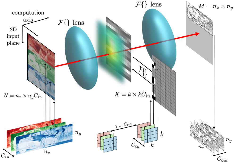
The diagram illustrates a computational pipeline for image transformation through an optical system, involving Fourier domain processing and feature extraction. It shows the flow of a 2D input image through two lenses (F{}) and intermediate processing stages, resulting in a multi-channel output image.
### Components/Axes
1. **Input Plane (2D Input Plane)**
- Dimensions: `N = nx × ny × Cin`
- Channels: Red (`C_in`), Green (`C_in`), Blue (`C_in`)
- Position: Bottom-left quadrant
- Visualization: Color image of a car split into RGB channels
2. **Fourier Plane (F{} Lens)**
- Dimensions: `K = k × k × C_in`
- Visualization: Blurred grid with intensity variations (green/yellow center)
- Position: Center of the diagram
- Legend: Gray grid representing spatial frequency domain
3. **Output Plane (M = nx × ny × C_out)**
- Dimensions: `M = nx × ny × C_out`
- Channels: `C_out` (multiple grayscale feature maps)
- Position: Right side of the diagram
- Visualization: Edge-detected car images with varying orientations
4. **Computation Axis**
- Red arrow connecting input → Fourier plane → output
- Indicates data flow direction
### Detailed Analysis
- **Input Plane**:
- RGB channels (`C_in`) are spatially aligned (`nx × ny` pixels)
- Color coding matches standard RGB convention (red/green/blue)
- **Fourier Plane**:
- Grid structure (`k × k`) suggests convolutional kernel size
- Intensity gradient (green/yellow center) implies frequency magnitude representation
- **Output Plane**:
- `C_out` channels show progressive edge detection (horizontal → vertical → diagonal)
- Spatial resolution preserved (`nx × ny`)
### Key Observations
1. **Channel Preservation**: Input channels (`C_in`) are maintained through the Fourier transformation
2. **Feature Multiplication**: Output channels (`C_out`) exceed input channels, indicating feature expansion
3. **Spatial Consistency**: Pixel dimensions (`nx × ny`) remain constant through all stages
4. **Kernel Size**: `k × k` grid in Fourier plane suggests localized frequency analysis
### Interpretation
This diagram represents a computational model for image feature extraction using optical system analogies:
1. **First Lens (F{})**: Performs Fourier transform to convert spatial domain image to frequency domain
2. **Fourier Plane Processing**: Implicit filtering occurs in frequency space (green/yellow gradient suggests high-pass filtering)
3. **Second Lens (F{})**: Inverse Fourier transform converts processed frequencies back to spatial domain
4. **Output Channels**: Multiple `C_out` channels demonstrate feature decomposition (e.g., edge detection in different orientations)
The system appears to implement a convolutional neural network architecture using optical metaphors, where:
- Input plane = Raw image data
- Fourier plane = Convolutional filter application in frequency domain
- Output plane = Feature maps after non-linear transformation
Notable design choices:
- Color coding for input channels aids in tracking data flow
- Grid visualization in Fourier plane emphasizes frequency localization
- Multiple output channels show hierarchical feature extraction