## Chart: Gradient Updates vs. Dimension
### Overview
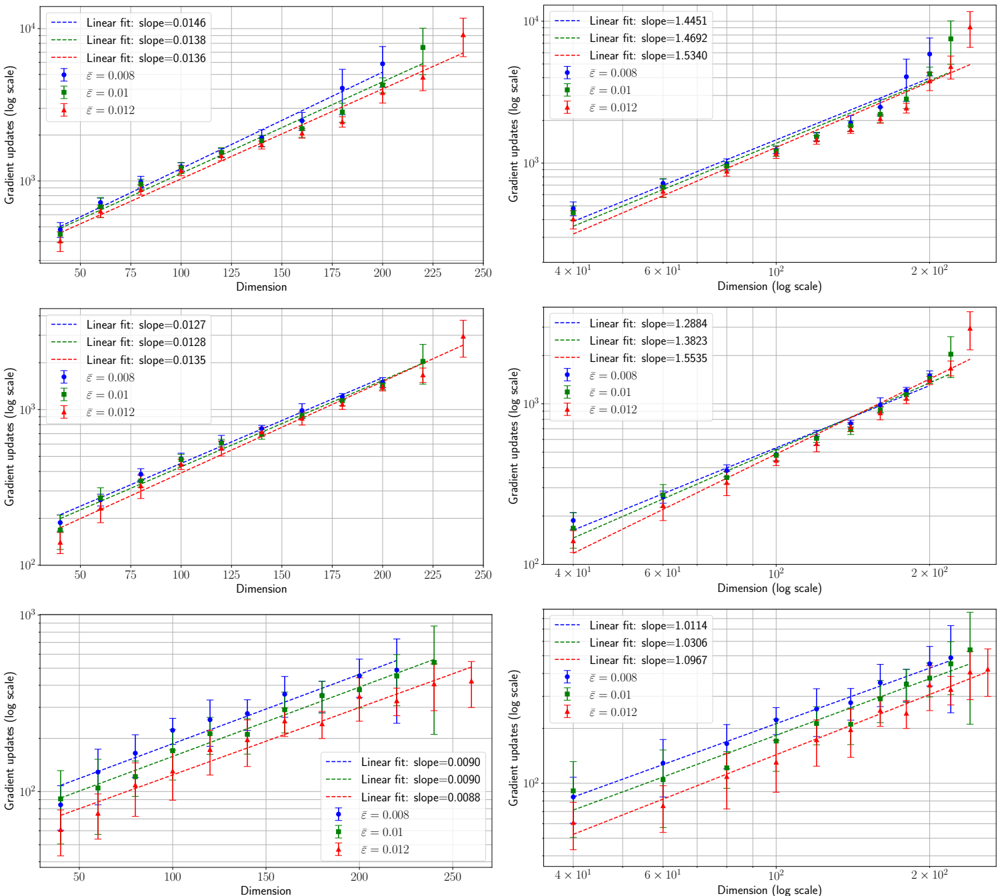
The image presents six scatter plots, each displaying the relationship between "Gradient updates (log scale)" and "Dimension". The plots are arranged in a 2x3 grid. Each plot shows data for three different values of epsilon (ε = 0.008, ε = 0.01, and ε = 0.012), along with linear fits for each epsilon value. The x-axis represents "Dimension," and the y-axis represents "Gradient updates (log scale)". The left column uses a linear scale for the x-axis, while the right column uses a logarithmic scale.
### Components/Axes
* **Y-axis (all plots):** "Gradient updates (log scale)". The scale ranges from approximately 10^2 to 10^4.
* **X-axis (left column):** "Dimension". The scale ranges from 50 to 250 in linear increments.
* **X-axis (right column):** "Dimension (log scale)". The scale ranges from approximately 4 x 10^1 to 2 x 10^2 in logarithmic increments.
* **Legend (all plots):** Located in the top-left corner of each plot.
* Blue: Linear fit for ε = 0.008
* Green: Linear fit for ε = 0.01
* Red: Linear fit for ε = 0.012
* Blue markers: ε = 0.008
* Green markers: ε = 0.01
* Red markers: ε = 0.012
### Detailed Analysis
**Top-Left Plot:**
* X-axis: Dimension (linear scale)
* Linear fit (blue, ε = 0.008): Slope = 0.0146. The blue data points increase approximately linearly from ~300 at dimension 50 to ~3000 at dimension 250.
* Linear fit (green, ε = 0.01): Slope = 0.0138. The green data points increase approximately linearly from ~400 at dimension 50 to ~2500 at dimension 250.
* Linear fit (red, ε = 0.012): Slope = 0.0136. The red data points increase approximately linearly from ~500 at dimension 50 to ~2500 at dimension 250.
**Top-Right Plot:**
* X-axis: Dimension (log scale)
* Linear fit (blue, ε = 0.008): Slope = 1.4451. The blue data points increase approximately linearly from ~300 at dimension 40 to ~8000 at dimension 200.
* Linear fit (green, ε = 0.01): Slope = 1.4692. The green data points increase approximately linearly from ~400 at dimension 40 to ~9000 at dimension 200.
* Linear fit (red, ε = 0.012): Slope = 1.5340. The red data points increase approximately linearly from ~500 at dimension 40 to ~12000 at dimension 200.
**Middle-Left Plot:**
* X-axis: Dimension (linear scale)
* Linear fit (blue, ε = 0.008): Slope = 0.0127. The blue data points increase approximately linearly from ~250 at dimension 50 to ~2000 at dimension 250.
* Linear fit (green, ε = 0.01): Slope = 0.0128. The green data points increase approximately linearly from ~300 at dimension 50 to ~2200 at dimension 250.
* Linear fit (red, ε = 0.012): Slope = 0.0135. The red data points increase approximately linearly from ~400 at dimension 50 to ~2500 at dimension 250.
**Middle-Right Plot:**
* X-axis: Dimension (log scale)
* Linear fit (blue, ε = 0.008): Slope = 1.2884. The blue data points increase approximately linearly from ~250 at dimension 40 to ~4000 at dimension 200.
* Linear fit (green, ε = 0.01): Slope = 1.3823. The green data points increase approximately linearly from ~300 at dimension 40 to ~6000 at dimension 200.
* Linear fit (red, ε = 0.012): Slope = 1.5535. The red data points increase approximately linearly from ~400 at dimension 40 to ~10000 at dimension 200.
**Bottom-Left Plot:**
* X-axis: Dimension (linear scale)
* Linear fit (blue, ε = 0.008): Slope = 0.0090. The blue data points increase approximately linearly from ~150 at dimension 50 to ~700 at dimension 250.
* Linear fit (green, ε = 0.01): Slope = 0.0090. The green data points increase approximately linearly from ~200 at dimension 50 to ~800 at dimension 250.
* Linear fit (red, ε = 0.012): Slope = 0.0088. The red data points increase approximately linearly from ~200 at dimension 50 to ~700 at dimension 250.
**Bottom-Right Plot:**
* X-axis: Dimension (log scale)
* Linear fit (blue, ε = 0.008): Slope = 1.0114. The blue data points increase approximately linearly from ~150 at dimension 40 to ~1500 at dimension 200.
* Linear fit (green, ε = 0.01): Slope = 1.0306. The green data points increase approximately linearly from ~200 at dimension 40 to ~2000 at dimension 200.
* Linear fit (red, ε = 0.012): Slope = 1.0967. The red data points increase approximately linearly from ~200 at dimension 40 to ~2500 at dimension 200.
### Key Observations
* In all plots, the gradient updates generally increase with dimension.
* The linear fits suggest a roughly linear relationship between dimension and gradient updates, especially when the x-axis is on a linear scale.
* The slopes of the linear fits vary across the different plots, indicating that the rate of increase in gradient updates with dimension depends on the specific scenario represented by each plot.
* The plots on the right (log scale for dimension) show a steeper increase in gradient updates compared to the plots on the left (linear scale for dimension), as indicated by the larger slope values.
* For a given dimension, a higher epsilon value generally corresponds to a higher gradient update value.
### Interpretation
The plots illustrate how gradient updates (on a log scale) change with increasing dimension for different values of epsilon. The use of both linear and logarithmic scales for the dimension axis provides different perspectives on the relationship. The logarithmic scale compresses the higher dimension values, making it easier to visualize the trend over a wider range.
The increasing gradient updates with dimension suggest that as the complexity of the model (represented by dimension) increases, the magnitude of the updates required during training also increases. The different slopes indicate that this relationship is not constant and depends on other factors.
The effect of epsilon is also notable. A higher epsilon value generally leads to larger gradient updates, which could be related to the learning rate or some other parameter influencing the training process.
The error bars on the data points indicate the variability or uncertainty in the gradient updates. The size of these error bars could provide insights into the stability and reliability of the training process.