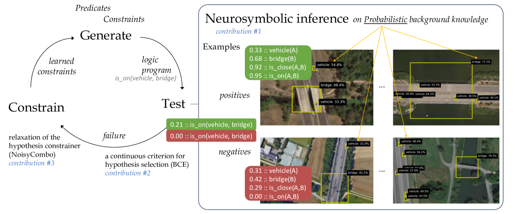
## System Diagram: Neurosymbolic Inference ### Overview The image presents a system diagram illustrating a neurosymbolic inference process. It combines symbolic reasoning (logic programs, constraints) with neural network outputs (probabilities associated with object detection). The diagram shows a cyclical process of generating hypotheses, testing them against examples, and constraining the hypothesis space based on the results. The right side of the diagram shows examples of positive and negative cases with object detection probabilities. ### Components/Axes * **Left Side (Process Flow)**: * **Generate**: Top of the cycle, associated with "Predicates" and "Constraints". An arrow points from "Generate" to "Test". * **Test**: Middle of the cycle. A "logic program is_on(vehicle, bridge)" is associated with this step. * **Constrain**: Bottom of the cycle, associated with "relaxation of the hypothesis constrainer (NoisyCombo) contribution #3". An arrow points from "Constrain" to "Generate", completing the cycle. * **Arrows**: Two curved arrows indicate the flow of information. One from "Generate" to "Test", and another from "Constrain" back to "Generate". A smaller arrow labeled "failure" points from "Test" to "Constrain". * **Right Side (Examples)**: * **Title**: "Neurosymbolic inference on Probabilistic background knowledge contribution #1" * **Examples**: Section header. * **Positives**: Labeled section containing examples where the "is_on(vehicle, bridge)" relationship is likely true. * **Negatives**: Labeled section containing examples where the "is_on(vehicle, bridge)" relationship is likely false. * **Images**: Several aerial images showing vehicles and bridges, with bounding boxes around detected objects. * **Probabilities**: Probabilities associated with object detections and relationships, displayed next to the images. ### Detailed Analysis or Content Details **Left Side (Process Flow)**: * **Generate**: This step involves generating hypotheses based on predicates and constraints. * **Test**: The generated hypotheses are tested using a logic program, specifically "is_on(vehicle, bridge)". * **Constrain**: Based on the test results, the hypothesis space is constrained. This involves relaxation of the hypothesis constrainer using a method called "NoisyCombo" (contribution #3). A continuous criterion for hypothesis selection (BCE) is also mentioned (contribution #2). * **Feedback Loop**: The process is cyclical, with the "Constrain" step feeding back into the "Generate" step, refining the hypotheses over time. **Right Side (Examples)**: * **Positive Examples**: * The first positive example shows the following probabilities: * 0.33 :: vehicle(A) * 0.68 :: bridge(B) * 0.92 :: is_close(A,B) * 0.95 :: is_on(A,B) * Image shows a bridge with vehicles on it. Bounding boxes are present around the vehicle and bridge. * vehicle: 54.8% * bridge: 68.4% * vehicle: 33.3% * The second positive example shows the following probabilities: * Image shows a bridge with vehicles on it. Bounding boxes are present around the vehicles and bridge. * bridge: 77.1% * vehicle: 55.5% * vehicle: 50.4% * vehicle: 64.2% * vehicle: 38.5% * vehicle: 48.1% * **Negative Examples**: * The first negative example shows the following probabilities: * 0.31 :: vehicle(A) * 0.42 :: bridge(B) * 0.29 :: is_close(A,B) * 0.00 :: is_on(A,B) * Image shows a bridge and a vehicle on a road next to the bridge. Bounding boxes are present around the vehicle and bridge. * vehicle: 31.0% * bridge: 42.2% * The second negative example shows the following probabilities: * Image shows a bridge and a vehicle on a road next to the bridge. Bounding boxes are present around the vehicles and bridge. * vehicle: 48.4% * vehicle: 56.2% * vehicle: 44.6% * vehicle: 57.0% * bridge: 79.1% * vehicle: 49.5% * vehicle: 43.5% * **Additional Notes**: * The probabilities represent the confidence of the model in detecting the objects and their relationships. * The positive examples have high probabilities for "is_on(A,B)", while the negative examples have low probabilities for "is_on(A,B)". * The green boxes "0.21 :: is_on(vehicle, bridge)" and "0.00 :: is_on(vehicle, bridge)" are used to show the result of the test. Green indicates success, red indicates failure. ### Key Observations * The diagram illustrates a neurosymbolic approach to reasoning about relationships between objects in images. * The system uses a feedback loop to refine its hypotheses based on positive and negative examples. * The probabilities associated with object detections play a crucial role in the inference process. * The "is_on(vehicle, bridge)" relationship is used as a specific example to demonstrate the system's capabilities. ### Interpretation The diagram demonstrates a system that combines neural networks and symbolic reasoning to infer relationships between objects in images. The cyclical process of generating, testing, and constraining hypotheses allows the system to learn and improve its accuracy over time. The use of probabilities from object detection provides a measure of confidence in the inferred relationships. The example of "is_on(vehicle, bridge)" shows how the system can be used to reason about spatial relationships between objects. The contributions #1, #2, and #3 likely refer to specific techniques or components used in the system, such as the neurosymbolic inference method, the hypothesis selection criterion, and the hypothesis constrainer.

## Neurosymbolic Inference Diagram: Probabilistic Logic Cycle with Visual Examples ### Overview This image is a technical diagram illustrating a neurosymbolic inference system that combines machine learning with logical reasoning. It depicts a cyclic process for generating and testing logical hypotheses against probabilistic visual data. The diagram is divided into two primary sections: a conceptual cycle on the left and a detailed panel on the right showing concrete examples of the inference process applied to aerial imagery. ### Components/Axes The diagram contains no traditional chart axes. Its components are: **Left Section - The Inference Cycle:** * **Three Core Nodes:** "Generate", "Test", "Constrain" arranged in a clockwise cycle. * **Connecting Arrows & Labels:** * From "Generate" to "Test": Arrow labeled "logic program" with sub-label `is_on(vehicle, bridge)`. * From "Test" to "Constrain": Arrow labeled "failure". * From "Constrain" to "Generate": Arrow labeled "learned constraints". * **Contributions (in blue italics):** * `contribution #1`: Associated with "Neurosymbolic inference on Probabilistic background knowledge". * `contribution #2`: Associated with "a continuous criterion for hypothesis selection (BCE)". * `contribution #3`: Associated with "relaxation of the hypothesis constrainer (NoisyCombo)". * **Additional Text:** "Predicates", "Constraints" at the top. **Right Section - Example Panel:** * **Title:** "Neurosymbolic inference on Probabilistic background knowledge" * **Sub-sections:** * **"Examples"**: Contains two green boxes listing probabilistic logical statements. * **"positives"**: Shows two aerial images with yellow bounding boxes and labels. * **"negatives"**: Shows two aerial images with yellow bounding boxes and labels. * **Visual Connectors:** Yellow arrows link the logical statements in the "Examples" boxes to specific bounding boxes in the "positives" and "negatives" images. ### Detailed Analysis **1. The Inference Cycle (Left Side):** The process is iterative: 1. **Generate:** Creates a logic program (e.g., `is_on(vehicle, bridge)`) based on predicates, constraints, and learned constraints from previous cycles. 2. **Test:** Evaluates the logic program against data. Two example outcomes are shown in colored boxes: * Green box: `0.21 :: is_on(vehicle, bridge)` * Red box: `0.00 :: is_on(vehicle, bridge)` The "failure" path is taken when the test yields a low probability (like 0.00). 3. **Constrain:** Uses the failure to relax or adjust the hypothesis constrainer (via "NoisyCombo", contribution #3), feeding back into the "Generate" step. **2. Probabilistic Examples (Right Side - "Examples" box):** * **Top Green Box (Positive Example):** * `0.33 :: vehicle(A)` * `0.68 :: bridge(B)` * `0.92 :: is_close(A,B)` * `0.95 :: is_on(A,B)` * **Bottom Red Box (Negative Example):** * `0.31 :: vehicle(A)` * `0.42 :: bridge(B)` * `0.29 :: is_close(A,B)` * `0.00 :: is_on(A,B)` **3. Visual Data with Bounding Boxes (Right Side - "positives"/"negatives"):** Each image contains multiple detected objects with confidence scores. The yellow arrows map the logical variables `A` and `B` from the examples to specific visual detections. * **Top-Left Positive Image:** * `vehicle: 54.8%` (arrow from `vehicle(A)`) * `bridge: 68.4%` (arrow from `bridge(B)`) * `vehicle: 33.3%` * **Top-Right Positive Image:** * `bridge: 77.1%` (arrow from `bridge(B)`) * `vehicle: 55.5%` (arrow from `vehicle(A)`) * `vehicle: 50.4%` * `vehicle: 64.2%` * `vehicle: 18.5%` * `vehicle: 85.1%` * **Bottom-Left Negative Image:** * `vehicle: 33.0%` (arrow from `vehicle(A)`) * `bridge: 42.2%` (arrow from `bridge(B)`) * **Bottom-Right Negative Image:** * `vehicle: 48.4%` (arrow from `vehicle(A)`) * `bridge: 79.1%` (arrow from `bridge(B)`) * `vehicle: 56.2%` * `vehicle: 66.8%` * `vehicle: 57.0%` * `vehicle: 39.3%` * `vehicle: 43.5%` ### Key Observations 1. **Probabilistic Logic:** The system does not use binary true/false but assigns probabilities (0.00 to 0.95) to logical statements, reflecting uncertainty in perception and reasoning. 2. **Positive vs. Negative Correlation:** In the "positives" examples, the `is_on(A,B)` statement has high probability (0.95), correlating with visual detections where a vehicle and bridge are spatially related. In the "negatives" example, `is_on(A,B)` has 0.00 probability, even though a vehicle and bridge are detected (with lower confidence: 31% and 42%). 3. **Spatial Grounding:** The yellow arrows explicitly ground abstract logical variables (`A`, `B`) to concrete pixel regions in the images, demonstrating the neurosymbolic link. 4. **Cycle Logic:** The "failure" path from "Test" to "Constrain" is triggered by low-probability outcomes (like the 0.00 result), which then informs the generation of new constraints to improve future hypotheses. ### Interpretation This diagram presents a framework for **robust visual reasoning under uncertainty**. It addresses a core challenge in AI: combining the pattern recognition strength of neural networks (which output probabilistic detections like `vehicle: 54.8%`) with the structured reasoning of symbolic logic (which can express relationships like `is_on`). * **How it Works:** The system generates a logical hypothesis (e.g., "there is a vehicle on a bridge"). It tests this hypothesis by checking if the underlying visual detections (vehicle, bridge) and their spatial relationship (`is_close`) are supported by the neural network's output with sufficient confidence. If the combined probability is too low (a "failure"), the system learns to adjust its constraining rules, making future hypotheses more plausible or better aligned with the data. * **Significance:** The "positives" and "negatives" show that the system isn't just checking for the presence of objects, but for a specific, complex relationship between them. The negative case is crucial—it shows a scenario where objects are detected but the critical relationship is not supported, leading to a logical rejection (`0.00 :: is_on`). * **Contributions:** The three labeled contributions highlight the novel components: 1) The core neurosymbolic inference method itself, 2) A continuous (non-binary) criterion (BCE - likely Binary Cross-Entropy) for selecting the best hypothesis, and 3) A specific technique ("NoisyCombo") for relaxing logical constraints when faced with failure, enabling learning and adaptation. In essence, the diagram illustrates a closed-loop system where visual perception informs logical reasoning, and logical failures guide the improvement of the reasoning process, all while quantitatively handling the inherent uncertainty of real-world data.

## Diagram: Neurosymbolic Inference System with Probabilistic Background Knowledge ### Overview The image depicts a hybrid neurosymbolic inference system combining logic programming with probabilistic reasoning. It features a cyclical process for hypothesis generation and testing, alongside visual examples of object detection in aerial imagery. The system uses probabilistic background knowledge to constrain hypothesis selection and iteratively refines constraints based on test failures. ### Components/Axes **Left Section (Flowchart):** - **Nodes:** - `Predicates` (top-left) - `Constraints` (top-center) - `Generate` (center) - `Test` (right-center) - `failure` (bottom-center) - **Arrows:** - `learned constraints` (from Constraints to Generate) - `logic program` (from Generate to Test) - `is_on(vehicle, bridge)` (example predicate) - `relaxation of the hypothesis constrainer (NoisyCombo)` (from failure back to Constraints) - **Labels:** - `contribution #1` (near "Neurosymbolic inference") - `contribution #2` (near "BCE") - `contribution #3` (near "NoisyCombo") **Right Section (Image Grid):** - **Images:** Four aerial photographs showing roads, bridges, and vehicles. - **Annotations:** - **Green boxes (positives):** - `0.33 :: vehicle(A)` - `0.68 :: bridge(B)` - `0.92 :: is_close(A,B)` - `0.95 :: is_on(A,B)` - **Red boxes (negatives):** - `0.21 :: is_on(vehicle, bridge)` - `0.00 :: is_on(vehicle, bridge)` - `0.31 :: vehicle(A)` - `0.42 :: bridge(B)` - `0.29 :: is_close(A,B)` - `0.00 :: is_on(A,B)` - **Legend:** - Green = positives - Red = negatives ### Detailed Analysis **Flowchart Process:** 1. **Hypothesis Generation:** Combines predicates (e.g., `is_on(vehicle, bridge)`) with learned constraints to produce logic programs. 2. **Testing:** Evaluates hypotheses against real-world data (aerial images). 3. **Failure Handling:** Relaxes constraints (via NoisyCombo) when tests fail, enabling iterative refinement. **Image Annotations:** - **Positive Examples (Green):** High-confidence detections (e.g., 0.95 for `is_on(A,B)`). - **Negative Examples (Red):** Low-confidence or incorrect predictions (e.g., 0.00 for `is_on(vehicle, bridge)`). - **Probabilistic Scores:** Percentages in bounding boxes (e.g., "vehicle: 54.8%") likely represent model confidence in detections. ### Key Observations 1. **Iterative Refinement:** The flowchart's cyclical nature suggests adaptive learning from failures. 2. **Confidence Thresholding:** Negative examples with 0.00 scores indicate strict filtering of low-confidence predictions. 3. **Spatial Relationships:** The `is_close` and `is_on` predicates highlight the system's ability to reason about object proximity and positioning. 4. **Probabilistic Grounding:** Percentages in images (e.g., "bridge: 77.1%") demonstrate integration of probabilistic background knowledge. ### Interpretation This system bridges symbolic logic (e.g., `is_on(vehicle, bridge)`) with probabilistic reasoning, enabling robust object detection in complex aerial imagery. The iterative constraint relaxation (NoisyCombo) addresses noisy real-world data, while the BCE (Binary Cross-Entropy) criterion ensures only high-confidence hypotheses are retained. The visual examples show the system's ability to detect vehicles and bridges with varying confidence, though some cases (e.g., 0.00 scores) reveal limitations in handling ambiguous scenarios. The integration of learned constraints with probabilistic background knowledge suggests a framework for improving generalization in uncertain environments.