## Chart Type: Line Plots
### Overview
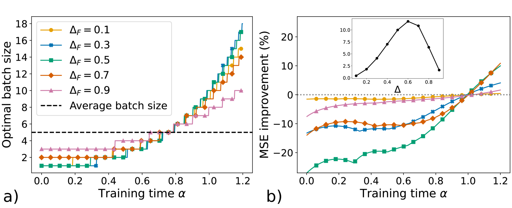
The image contains two line plots, labeled a) and b), that explore the relationship between training time and optimal batch size, and training time and MSE improvement, respectively. The plots analyze the impact of different values of ΔF on these relationships. Plot b) also contains an inset plot showing the relationship between Δ and an unspecified variable.
### Components/Axes
**Plot a)**
* **Title:** Optimal batch size vs. Training time α
* **X-axis:** Training time α, with values ranging from 0.0 to 1.2 in increments of 0.2.
* **Y-axis:** Optimal batch size, with values ranging from 2 to 18 in increments of 2.
* **Legend (Top-Left):**
* Yellow line with circles: ΔF = 0.1
* Blue line with diamonds: ΔF = 0.3
* Green line with squares: ΔF = 0.5
* Orange line with diamonds: ΔF = 0.7
* Pink line with triangles: ΔF = 0.9
* Black dashed line: Average batch size
**Plot b)**
* **Title:** MSE improvement (%) vs. Training time α
* **X-axis:** Training time α, with values ranging from 0.0 to 1.2 in increments of 0.2.
* **Y-axis:** MSE improvement (%), with values ranging from -20 to 20 in increments of 10.
* **Legend:** Same as Plot a).
* **Horizontal dotted line:** Represents 0% MSE improvement.
**Inset Plot (Plot b)**
* **X-axis:** Δ, with values ranging from 0.0 to 0.8 in increments of 0.2.
* **Y-axis:** Unspecified, with values ranging from 0.0 to 10.0 in increments of 2.5.
### Detailed Analysis
**Plot a) - Optimal batch size**
* **Average batch size (Black dashed line):** Constant at approximately 5.
* **ΔF = 0.1 (Yellow line with circles):** Remains relatively constant at approximately 2 until α ≈ 0.8, then increases stepwise to approximately 15 at α = 1.2.
* **ΔF = 0.3 (Blue line with diamonds):** Remains relatively constant at approximately 1 until α ≈ 0.8, then increases stepwise to approximately 16 at α = 1.2.
* **ΔF = 0.5 (Green line with squares):** Remains relatively constant at approximately 1 until α ≈ 0.8, then increases stepwise to approximately 15 at α = 1.2.
* **ΔF = 0.7 (Orange line with diamonds):** Remains relatively constant at approximately 2 until α ≈ 0.8, then increases stepwise to approximately 14 at α = 1.2.
* **ΔF = 0.9 (Pink line with triangles):** Remains relatively constant at approximately 3 until α ≈ 0.8, then increases stepwise to approximately 9 at α = 1.2.
**Plot b) - MSE improvement**
* **ΔF = 0.1 (Yellow line with circles):** Remains relatively constant at approximately -2% throughout the training time.
* **ΔF = 0.3 (Blue line with diamonds):** Starts at approximately -12% and gradually increases to approximately 2% at α = 1.2.
* **ΔF = 0.5 (Green line with squares):** Starts at approximately -24% and increases sharply to approximately 12% at α = 1.2.
* **ΔF = 0.7 (Orange line with diamonds):** Starts at approximately -14% and increases to approximately 12% at α = 1.2.
* **ΔF = 0.9 (Pink line with triangles):** Starts at approximately -7% and increases slightly to approximately 2% at α = 1.2.
**Inset Plot (Plot b)**
* The black line increases from approximately 0 at Δ = 0.0 to a peak of approximately 11 at Δ = 0.6, then decreases to approximately 3 at Δ = 0.8.
### Key Observations
* In Plot a), the optimal batch size remains relatively constant for all ΔF values until a training time of approximately 0.8, after which it increases sharply.
* In Plot b), the MSE improvement varies significantly depending on the ΔF value. Lower ΔF values (0.1 and 0.9) result in relatively constant or slightly increasing MSE improvement, while higher ΔF values (0.3, 0.5, and 0.7) show a more significant increase in MSE improvement as training time increases.
* The inset plot in Plot b) shows a non-linear relationship between Δ and the unspecified variable, with a peak at Δ = 0.6.
### Interpretation
The plots suggest that the optimal batch size is relatively stable during the initial stages of training, but increases significantly as training progresses beyond a certain point (α ≈ 0.8). The value of ΔF has a significant impact on the MSE improvement, with higher values generally leading to greater improvements, especially at later stages of training. The inset plot indicates that there is an optimal value of Δ (around 0.6) for maximizing some other performance metric, which is not explicitly defined in the plot. The relationship between Δ and ΔF is not clear from the plots, but it is possible that they are related.