\n
## Line Graph: Negative Logarithm of One Plus Exponential Function
### Overview
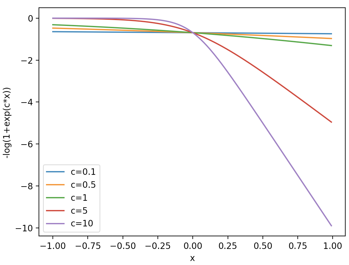
The image is a 2D line graph plotting the mathematical function `-log(1+exp(c*x))` against the variable `x` for five different values of the parameter `c`. The graph demonstrates how the shape of this function changes as the scaling factor `c` increases.
### Components/Axes
* **X-Axis:**
* **Label:** `x`
* **Range:** -1.00 to 1.00
* **Major Tick Marks:** -1.00, -0.75, -0.50, -0.25, 0.00, 0.25, 0.50, 0.75, 1.00
* **Y-Axis:**
* **Label:** `-log(1+exp(c*x))`
* **Range:** Approximately -10 to 0
* **Major Tick Marks:** -10, -8, -6, -4, -2, 0
* **Legend:**
* **Position:** Bottom-left corner of the plot area.
* **Content:** A list of five colored lines with corresponding parameter values.
* **Entries (from top to bottom in legend):**
1. Blue line: `c=0.1`
2. Orange line: `c=0.5`
3. Green line: `c=1`
4. Red line: `c=5`
5. Purple line: `c=10`
### Detailed Analysis
The graph displays five distinct curves, each corresponding to a different `c` value. All curves intersect at the point (0, -log(2)) ≈ (0, -0.693).
1. **c=0.1 (Blue Line):**
* **Trend:** Nearly horizontal, with a very slight downward slope.
* **Data Points (Approximate):** At x=-1.00, y ≈ -0.65. At x=1.00, y ≈ -0.75. The line remains close to y = -0.7 across the entire domain.
2. **c=0.5 (Orange Line):**
* **Trend:** Gentle, consistent downward slope.
* **Data Points (Approximate):** At x=-1.00, y ≈ -0.55. At x=1.00, y ≈ -0.95.
3. **c=1 (Green Line):**
* **Trend:** Moderate downward slope, steeper than the c=0.5 line.
* **Data Points (Approximate):** At x=-1.00, y ≈ -0.35. At x=1.00, y ≈ -1.35.
4. **c=5 (Red Line):**
* **Trend:** For negative x, the line is nearly flat and close to y=0. After x=0, it slopes downward steeply and linearly.
* **Data Points (Approximate):** At x=-1.00, y ≈ -0.01. At x=0.00, y ≈ -0.69. At x=1.00, y ≈ -5.0.
5. **c=10 (Purple Line):**
* **Trend:** Similar to the c=5 line but with a more extreme transition. It is flat near y=0 for negative x and then plummets with a very steep, linear downward slope for positive x.
* **Data Points (Approximate):** At x=-1.00, y ≈ -0.00005 (effectively 0). At x=0.00, y ≈ -0.69. At x=1.00, y ≈ -10.0.
### Key Observations
* **Intersection Point:** All five curves pass through the same point at x=0, where the function value is `-log(2)`.
* **Effect of Parameter `c`:** As `c` increases, the function's behavior bifurcates. For negative `x`, higher `c` values make the function approach 0. For positive `x`, higher `c` values cause the function to decrease (become more negative) much more rapidly.
* **Linearity for Positive x:** For `c=5` and `c=10`, the function appears to become linear for `x > 0`, with a slope approximately equal to `-c`.
* **Symmetry Breaking:** The function is not symmetric around x=0. The asymmetry becomes dramatically more pronounced as `c` increases.
### Interpretation
This graph visualizes the behavior of a function commonly encountered in statistics and machine learning, often related to loss functions (like the logistic loss) or softplus functions. The parameter `c` acts as a scaling or "sharpness" factor.
* **Low `c` (0.1, 0.5, 1):** The function is smooth and changes gradually across the entire domain of `x`. It provides a gentle penalty that increases as `x` moves away from zero in either direction.
* **High `c` (5, 10):** The function approximates a "hinge" or a rectifier. It is essentially zero (no penalty) for all negative inputs (`x < 0`) and then imposes a severe, linear penalty for positive inputs (`x > 0`). This mimics behavior like a ReLU activation or a hard margin loss, where only one side of the input space is penalized.
The plot effectively demonstrates how a single mathematical form can transition from a smooth, symmetric-like function to a sharp, asymmetric one simply by adjusting a scaling parameter. This is crucial for understanding model behavior in optimization contexts, where `c` might control the trade-off between margin and loss.