## Chart Type: Density and Cumulative Distribution Plots
### Overview
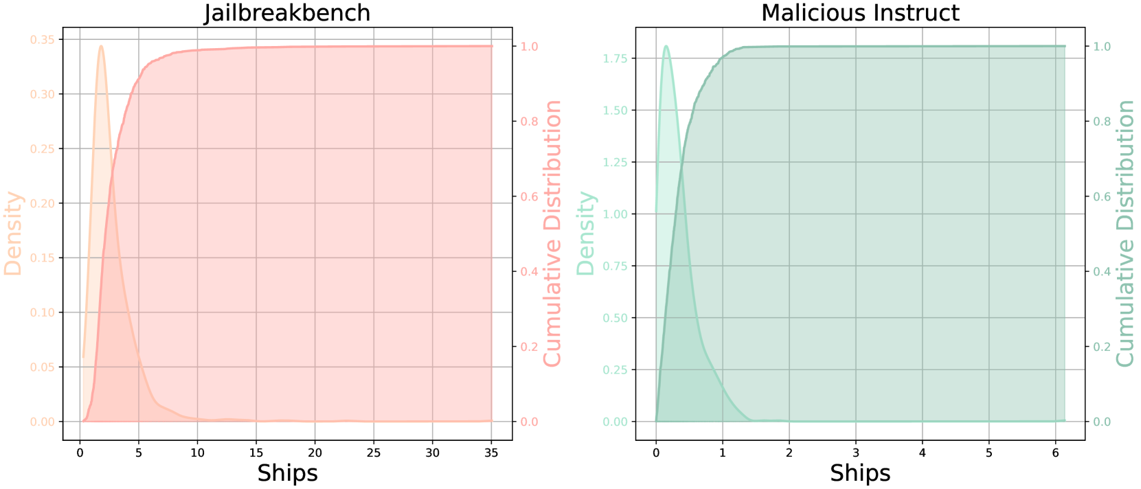
The image presents two plots side-by-side, each displaying a density curve and a cumulative distribution curve. The left plot is titled "Jailbreakbench," and the right plot is titled "Malicious Instruct." Both plots share a similar structure with density on the left y-axis and cumulative distribution on the right y-axis, plotted against "Ships" on the x-axis.
### Components/Axes
**Left Plot (Jailbreakbench):**
* **Title:** Jailbreakbench
* **X-axis:** Ships, ranging from 0 to 35 in increments of 5.
* **Left Y-axis:** Density, ranging from 0.00 to 0.35 in increments of 0.05.
* **Right Y-axis:** Cumulative Distribution, ranging from 0.0 to 1.0 in increments of 0.2.
* **Density Curve:** Light orange color.
* **Cumulative Distribution Curve:** Light red color.
**Right Plot (Malicious Instruct):**
* **Title:** Malicious Instruct
* **X-axis:** Ships, ranging from 0 to 6 in increments of 1.
* **Left Y-axis:** Density, ranging from 0.00 to 1.75 in increments of 0.25.
* **Right Y-axis:** Cumulative Distribution, ranging from 0.0 to 1.0 in increments of 0.2.
* **Density Curve:** Light green color.
* **Cumulative Distribution Curve:** Light teal color.
### Detailed Analysis
**Left Plot (Jailbreakbench):**
* **Density Curve (Light Orange):**
* The density curve peaks sharply around x = 1, reaching a density of approximately 0.34.
* It then rapidly decreases, approaching 0 for x > 5.
* **Cumulative Distribution Curve (Light Red):**
* The cumulative distribution starts at 0 and rapidly increases until approximately x = 10.
* It then gradually approaches 1, reaching a value close to 1 for x > 20.
* At x = 5, the cumulative distribution is approximately 0.25.
* At x = 10, the cumulative distribution is approximately 0.33.
* At x = 15, the cumulative distribution is approximately 0.34.
**Right Plot (Malicious Instruct):**
* **Density Curve (Light Green):**
* The density curve peaks sharply around x = 0.25, reaching a density of approximately 1.75.
* It then rapidly decreases, approaching 0 for x > 1.
* **Cumulative Distribution Curve (Light Teal):**
* The cumulative distribution starts at 0 and rapidly increases until approximately x = 1.
* It then gradually approaches 1, reaching a value close to 1 for x > 2.
* At x = 0.5, the cumulative distribution is approximately 0.75.
* At x = 1, the cumulative distribution is approximately 0.95.
* At x = 2, the cumulative distribution is approximately 1.0.
### Key Observations
* Both plots show a rapid increase in the cumulative distribution at low "Ships" values, indicating that most of the data is concentrated in this region.
* The "Jailbreakbench" plot has a wider distribution compared to the "Malicious Instruct" plot, as indicated by the x-axis ranges (0-35 vs. 0-6).
* The density curve for "Malicious Instruct" is much higher and narrower than that of "Jailbreakbench," suggesting a higher concentration of data around a smaller range of "Ships."
### Interpretation
The plots compare the distribution of "Ships" for "Jailbreakbench" and "Malicious Instruct." The "Jailbreakbench" data is more spread out, with a lower density peak, indicating a wider range of "Ships" values. In contrast, "Malicious Instruct" has a much higher density peak at a very low "Ships" value, indicating that most instances involve a very small number of "Ships." The cumulative distribution curves show how quickly the data accumulates; "Malicious Instruct" reaches its maximum cumulative distribution much faster than "Jailbreakbench." This suggests that "Malicious Instruct" is more likely to involve fewer "Ships" compared to "Jailbreakbench."