## Diagram: Neural Network Block Architecture
### Overview
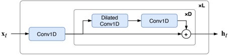
The image illustrates a modular neural network architecture block, commonly used in sequence modeling (such as WaveNet or Temporal Convolutional Networks). The diagram depicts a signal flow that incorporates an initial convolution, a residual branch containing a dilated convolution, and a summation operation. The structure is nested, indicating that specific components are repeated $D$ times and the entire block is repeated $L$ times.
### Components/Axes
* **Input/Output:**
* **$x_t$**: The input signal, entering from the left.
* **$h_t$**: The output signal, exiting to the right.
* **Processing Blocks (Blue Rectangles):**
* **Conv1D (Left):** The initial 1D convolution layer.
* **Dilated Conv1D (Top-Center):** A 1D convolution layer with dilation, located inside the inner box.
* **Conv1D (Top-Right):** A standard 1D convolution layer, located inside the inner box, following the Dilated Conv1D.
* **Operations:**
* **$\oplus$ (Summation Node):** Located on the right side, this node adds the output of the processing path to the residual path.
* **Containers/Multipliers:**
* **Inner Box (labeled "xD"):** Encloses the "Dilated Conv1D" and the second "Conv1D" block. This indicates that this specific sequence of operations is repeated $D$ times.
* **Outer Box (labeled "xL"):** Encloses the entire architecture, including the initial "Conv1D" and the "xD" box. This indicates that the entire block structure is repeated $L$ times.
### Detailed Analysis
The flow of data through the diagram is as follows:
1. **Initial Processing:** The input $x_t$ enters the first "Conv1D" block.
2. **Branching:** Upon exiting the first "Conv1D" block, the signal path splits:
* **Residual Path (Bottom):** A direct, horizontal line connects the output of the first "Conv1D" directly to the summation node ($\oplus$). This is a "skip connection."
* **Processing Path (Top):** The signal enters the inner box ("xD"). It passes through the "Dilated Conv1D" block, then flows into the second "Conv1D" block.
3. **Recombination:** The output of the processing path (from the second "Conv1D") is directed downward into the summation node ($\oplus$), where it is added to the signal from the residual path.
4. **Output:** The result of the summation is the output $h_t$.
### Key Observations
* **Residual Learning:** The presence of the direct line bypassing the "Dilated Conv1D" and "Conv1D" blocks indicates a residual connection, which is a standard technique to facilitate the training of deeper networks by allowing gradients to flow more easily.
* **Receptive Field Expansion:** The use of "Dilated Conv1D" suggests the architecture is designed to increase the receptive field of the network (the amount of input data the network "sees" at once) without significantly increasing the number of parameters.
* **Scalability:** The labels "xD" and "xL" explicitly define the scalability of the architecture. The network depth can be adjusted by changing $L$, and the complexity of the dilated processing can be adjusted by changing $D$.
### Interpretation
This diagram represents a fundamental building block for deep temporal models. The architecture is designed to process sequential data ($x_t$) while maintaining the ability to learn long-range dependencies.
The "Dilated Conv1D" is the critical component here; by skipping input values (dilation), the network can capture patterns over a longer time horizon than a standard convolution would allow with the same kernel size. The residual connection (the skip connection) is essential for the "xL" scaling—without it, stacking many layers (large $L$) would likely lead to vanishing gradients, making the model impossible to train. The structure suggests a highly efficient, hierarchical feature extractor where the model learns to combine local features (via the initial Conv1D) with broader temporal context (via the Dilated Conv1D).