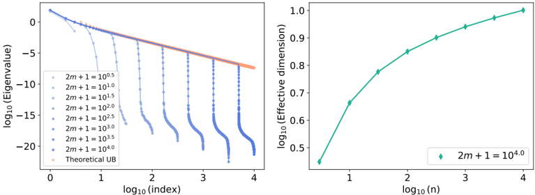
\n ## Charts: Eigenvalue Spectrum and Effective Dimension ### Overview The image presents two charts. The left chart displays the log10 of the Eigenvalue versus the log10 of the index for different values of `2m+1`. The right chart shows the log10 of the Effective Dimension versus the log10 of n, for a single value of `2m+1`. ### Components/Axes **Left Chart:** * **X-axis:** `log10(Index)` ranging from approximately 0 to 4. * **Y-axis:** `log10(Eigenvalue)` ranging from approximately 0 to -20. * **Data Series:** Multiple lines representing different values of `2m+1`: `10^5`, `10^4`, `10^3`, `10^2`, `10^1`, `10^0`. * **Additional Line:** A line labeled "Theoretical UB" (Upper Bound). * **Legend:** Located in the top-left corner, listing the values of `2m+1` and "Theoretical UB" with corresponding colors. **Right Chart:** * **X-axis:** `log10(n)` ranging from approximately 0 to 4. * **Y-axis:** `log10(Effective dimension)` ranging from approximately 0.5 to 1.0. * **Data Series:** A single line with markers representing data points for `2m+1 = 10^6`. * **Legend:** Located in the bottom-right corner, indicating `2m+1 = 10^6` with a teal color. ### Detailed Analysis or Content Details **Left Chart:** * **`2m+1 = 10^5` (Dark Blue):** The line starts at approximately `log10(Eigenvalue) = 0` at `log10(Index) = 0` and decreases steadily to approximately `log10(Eigenvalue) = -18` at `log10(Index) = 4`. * **`2m+1 = 10^4` (Blue):** The line starts at approximately `log10(Eigenvalue) = 0` at `log10(Index) = 0` and decreases steadily to approximately `log10(Eigenvalue) = -16` at `log10(Index) = 4`. * **`2m+1 = 10^3` (Light Blue):** The line starts at approximately `log10(Eigenvalue) = 0` at `log10(Index) = 0` and decreases steadily to approximately `log10(Eigenvalue) = -14` at `log10(Index) = 4`. * **`2m+1 = 10^2` (Medium Blue):** The line starts at approximately `log10(Eigenvalue) = 0` at `log10(Index) = 0` and decreases steadily to approximately `log10(Eigenvalue) = -12` at `log10(Index) = 4`. * **`2m+1 = 10^1` (Blue):** The line starts at approximately `log10(Eigenvalue) = 0` at `log10(Index) = 0` and decreases steadily to approximately `log10(Eigenvalue) = -10` at `log10(Index) = 4`. * **`2m+1 = 10^0` (Orange):** The line starts at approximately `log10(Eigenvalue) = 0` at `log10(Index) = 0` and decreases steadily to approximately `log10(Eigenvalue) = -8` at `log10(Index) = 4`. * **Theoretical UB (Gray):** The line starts at approximately `log10(Eigenvalue) = 0` at `log10(Index) = 0` and decreases steadily to approximately `log10(Eigenvalue) = -6` at `log10(Index) = 4`. **Right Chart:** * **`2m+1 = 10^6` (Teal):** The line starts at approximately `log10(Effective dimension) = 0.5` at `log10(n) = 0` and increases to approximately `log10(Effective dimension) = 0.98` at `log10(n) = 4`. The line exhibits a curved, increasing trend. Specific data points (approximate): * `log10(n) = 1`: `log10(Effective dimension) = 0.65` * `log10(n) = 2`: `log10(Effective dimension) = 0.78` * `log10(n) = 3`: `log10(Effective dimension) = 0.90` ### Key Observations * In the left chart, as `2m+1` increases, the rate of decrease in `log10(Eigenvalue)` slows down. * The "Theoretical UB" line consistently lies above all the other lines in the left chart. * In the right chart, the effective dimension increases with `n`, approaching 1 as `n` increases. ### Interpretation The left chart illustrates the eigenvalue spectrum for different values of `2m+1`. The decreasing trend of the eigenvalues suggests a diminishing contribution from higher-order components. The "Theoretical UB" provides an upper bound on the eigenvalue distribution. The fact that the rate of decrease slows down with increasing `2m+1` suggests that larger values of `2m+1` lead to a more persistent contribution from higher-order components. The right chart shows how the effective dimension grows with `n`. The effective dimension represents the number of independent components needed to represent the data. As `n` increases, the effective dimension approaches 1, indicating that the data becomes increasingly concentrated in a lower-dimensional space. This suggests that the system is becoming more predictable or less complex as `n` increases. The relationship between the two charts is that the eigenvalue spectrum (left) influences the effective dimension (right). A slower decay of eigenvalues implies a higher effective dimension for a given `n`. The charts together provide insight into the dimensionality and complexity of the system being analyzed.