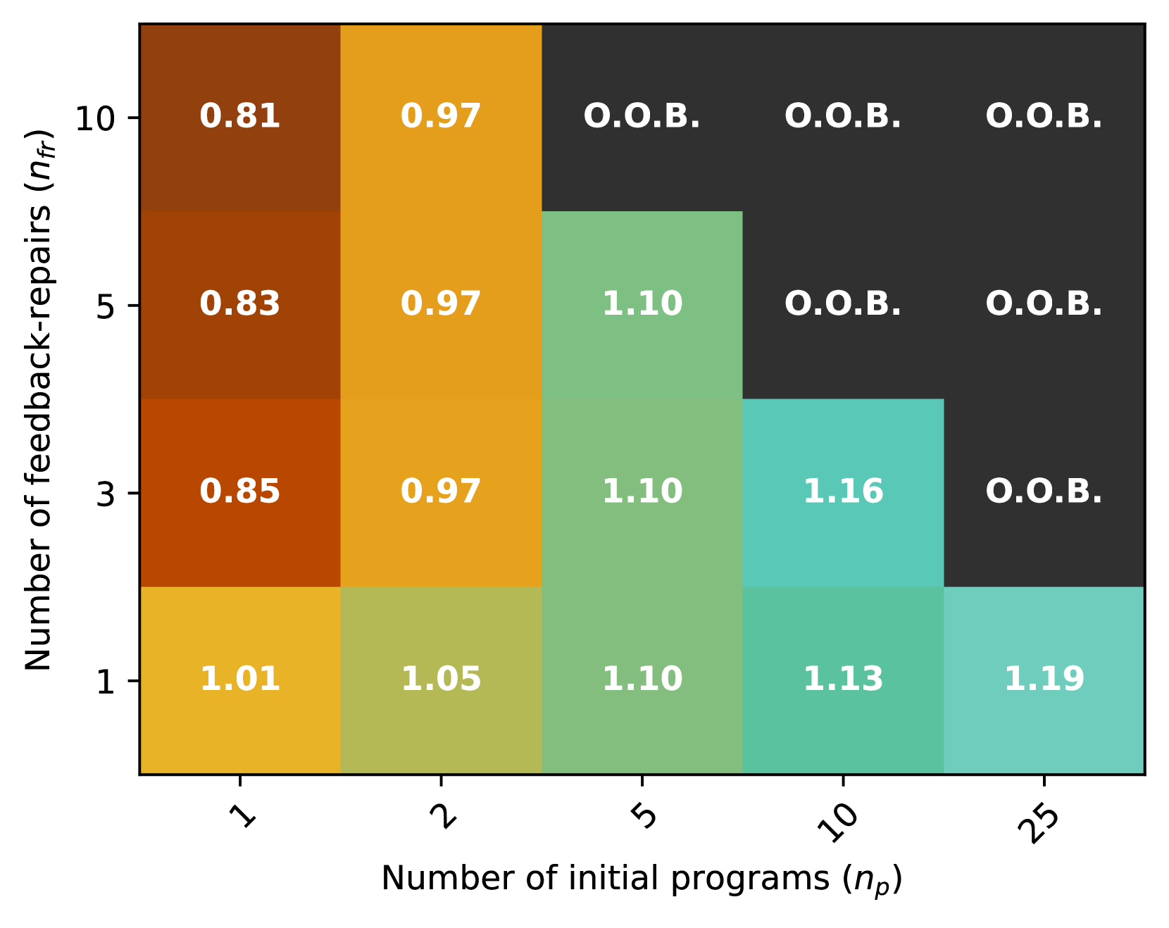
## Heatmap: Performance Metrics based on Feedback-Repairs and Initial Programs ### Overview This image displays a heatmap illustrating the relationship between two parameters, "Number of feedback-repairs ($n_{fr}$)" and "Number of initial programs ($n_P$)", and a measured outcome represented by numerical values within the cells. The color of each cell indicates the magnitude of the outcome, with a gradient from darker browns/reds (lower values) to greens and blues/teals (higher values). Some cells are marked "O.O.B." (Out Of Bounds) and are colored dark grey/black, indicating that no valid data was obtained for those parameter combinations. ### Components/Axes The chart is a 2D grid, or heatmap, with the following axes and labels: * **Y-axis (Vertical, left side):** * Label: "Number of feedback-repairs ($n_{fr}$)" * Tick Markers (from bottom to top): 1, 3, 5, 10 * **X-axis (Horizontal, bottom side):** * Label: "Number of initial programs ($n_P$)" * Tick Markers (from left to right): 1, 2, 5, 10, 25 * **Data Cells:** The grid consists of 4 rows (corresponding to $n_{fr}$ values) and 5 columns (corresponding to $n_P$ values), totaling 20 cells. Each cell contains a numerical value (e.g., 0.81, 1.10) or the text "O.O.B.". The text within the cells is white. * **Color Gradient (Implicit Legend):** * Darker brown/reddish-brown colors represent lower values (e.g., 0.81, 0.83, 0.85). * Orange/yellow-orange colors represent intermediate-low values (e.g., 0.97, 1.01). * Olive green/yellow-green colors represent slightly higher intermediate values (e.g., 1.05). * Light green/mint green colors represent intermediate-high values (e.g., 1.10). * Light blue/teal colors represent higher values (e.g., 1.13, 1.16, 1.19). * Dark grey/black color represents "O.O.B." (Out Of Bounds) entries. ### Detailed Analysis The heatmap presents a 4x5 matrix of values: | $n_{fr}$ \ $n_P$ | 1 | 2 | 5 | 10 | 25 | | :--------------- | :------- | :------- | :------- | :------- | :------- | | **10** | 0.81 | 0.97 | O.O.B. | O.O.B. | O.O.B. | | **5** | 0.83 | 0.97 | 1.10 | O.O.B. | O.O.B. | | **3** | 0.85 | 0.97 | 1.10 | 1.16 | O.O.B. | | **1** | 1.01 | 1.05 | 1.10 | 1.13 | 1.19 | **Row-wise Trends (increasing $n_P$ for fixed $n_{fr}$):** * **$n_{fr} = 10$ (Top Row):** * Starts at 0.81 (dark brown) for $n_P=1$. * Increases to 0.97 (orange) for $n_P=2$. * Becomes O.O.B. (dark grey/black) for $n_P=5, 10, 25$. * *Trend:* Values increase then become Out Of Bounds. * **$n_{fr} = 5$ (Second Row):** * Starts at 0.83 (brown) for $n_P=1$. * Increases to 0.97 (orange) for $n_P=2$. * Increases to 1.10 (light green) for $n_P=5$. * Becomes O.O.B. (dark grey/black) for $n_P=10, 25$. * *Trend:* Values increase then become Out Of Bounds. * **$n_{fr} = 3$ (Third Row):** * Starts at 0.85 (orange-brown) for $n_P=1$. * Increases to 0.97 (orange) for $n_P=2$. * Increases to 1.10 (light green) for $n_P=5$. * Increases to 1.16 (light blue/teal) for $n_P=10$. * Becomes O.O.B. (dark grey/black) for $n_P=25$. * *Trend:* Values consistently increase then become Out Of Bounds. * **$n_{fr} = 1$ (Bottom Row):** * Starts at 1.01 (yellow-orange) for $n_P=1$. * Increases to 1.05 (olive green) for $n_P=2$. * Increases to 1.10 (light green) for $n_P=5$. * Increases to 1.13 (light blue/teal) for $n_P=10$. * Increases to 1.19 (light blue/teal) for $n_P=25$. * *Trend:* Values consistently increase across all $n_P$ values, without encountering O.O.B. **Column-wise Trends (decreasing $n_{fr}$ for fixed $n_P$):** * **$n_P = 1$ (First Column):** * Starts at 0.81 ($n_{fr}=10$, dark brown). * Increases to 0.83 ($n_{fr}=5$, brown). * Increases to 0.85 ($n_{fr}=3$, orange-brown). * Increases to 1.01 ($n_{fr}=1$, yellow-orange). * *Trend:* Values consistently increase as $n_{fr}$ decreases. * **$n_P = 2$ (Second Column):** * Starts at 0.97 ($n_{fr}=10$, orange). * Remains 0.97 ($n_{fr}=5$, orange). * Remains 0.97 ($n_{fr}=3$, orange). * Increases to 1.05 ($n_{fr}=1$, olive green). * *Trend:* Values are constant for higher $n_{fr}$ then increase for the lowest $n_{fr}$. * **$n_P = 5$ (Third Column):** * Starts at O.O.B. ($n_{fr}=10$, dark grey/black). * Becomes 1.10 ($n_{fr}=5$, light green). * Remains 1.10 ($n_{fr}=3$, light green). * Remains 1.10 ($n_{fr}=1$, light green). * *Trend:* O.O.B. for highest $n_{fr}$, then constant value for lower $n_{fr}$. * **$n_P = 10$ (Fourth Column):** * Starts at O.O.B. ($n_{fr}=10$, dark grey/black). * Remains O.O.B. ($n_{fr}=5$, dark grey/black). * Becomes 1.16 ($n_{fr}=3$, light blue/teal). * Decreases slightly to 1.13 ($n_{fr}=1$, light blue/teal). * *Trend:* O.O.B. for higher $n_{fr}$, then a value appears and slightly decreases. * **$n_P = 25$ (Fifth Column):** * Starts at O.O.B. ($n_{fr}=10$, dark grey/black). * Remains O.O.B. ($n_{fr}=5$, dark grey/black). * Remains O.O.B. ($n_{fr}=3$, dark grey/black). * Becomes 1.19 ($n_{fr}=1$, light blue/teal). * *Trend:* O.O.B. for all but the lowest $n_{fr}$, where a high value appears. ### Key Observations * **O.O.B. Region:** A significant portion of the top-right of the heatmap is marked "O.O.B.". This region corresponds to combinations where both $n_{fr}$ and $n_P$ are relatively high. Specifically, for $n_{fr}=10$, any $n_P \ge 5$ is O.O.B. For $n_{fr}=5$, any $n_P \ge 10$ is O.O.B. For $n_{fr}=3$, $n_P=25$ is O.O.B. Only for $n_{fr}=1$ are all $n_P$ values within bounds. * **Value Range:** The observed numerical values range from a minimum of 0.81 to a maximum of 1.19. * **Inverse Relationship with $n_{fr}$ (for low $n_P$):** For $n_P=1$ and $n_P=2$, the outcome values generally increase as $n_{fr}$ decreases. * **Direct Relationship with $n_P$ (for low $n_{fr}$):** For $n_{fr}=1$, the outcome values consistently increase as $n_P$ increases. * **Lowest Value:** The lowest value (0.81) is found at the top-left corner ($n_{fr}=10, n_P=1$). * **Highest Value:** The highest value (1.19) is found at the bottom-right corner of the non-O.O.B. region ($n_{fr}=1, n_P=25$). * **Constant Values:** For $n_P=2$, the value is consistently 0.97 for $n_{fr}=10, 5, 3$. For $n_P=5$, the value is consistently 1.10 for $n_{fr}=5, 3, 1$. ### Interpretation The heatmap suggests that the measured outcome is sensitive to both the number of feedback-repairs ($n_{fr}$) and the number of initial programs ($n_P$). 1. **Optimal Region for Lower Values:** The lowest outcome values (represented by brown/red colors) are achieved when the number of feedback-repairs ($n_{fr}$) is high and the number of initial programs ($n_P$) is low. This implies that if the goal is to minimize this outcome, one should aim for a high $n_{fr}$ and low $n_P$. 2. **Optimal Region for Higher Values:** Conversely, the highest outcome values (represented by blue/teal colors) are achieved when $n_{fr}$ is low and $n_P$ is high. If maximizing this outcome is desired, a low $n_{fr}$ and high $n_P$ would be preferred. 3. **System Stability/Applicability (O.O.B. region):** The "O.O.B." entries indicate a region of parameter space where the system or experiment either failed to produce a result, or the conditions were outside a valid operating range. This suggests that increasing both $n_{fr}$ and $n_P$ simultaneously beyond certain thresholds leads to an unstable or undefined state. Specifically, high $n_{fr}$ values are more prone to O.O.B. conditions as $n_P$ increases. Only when $n_{fr}$ is at its minimum (1) can the system handle the maximum $n_P$ (25) without going O.O.B. This could imply resource limitations, computational complexity, or a breakdown in the underlying model or process. 4. **Trade-offs and Interactions:** There's a clear interaction between $n_{fr}$ and $n_P$. For instance, at $n_P=1$, increasing $n_{fr}$ significantly decreases the outcome. However, at $n_{fr}=1$, increasing $n_P$ significantly increases the outcome. The "O.O.B." boundary acts as a critical constraint, defining the feasible operating region for the system. Understanding the nature of "O.O.B." is crucial for practical application, as it delineates where the system's behavior becomes unpredictable or invalid.