## Line Graphs: Computational Efficiency (CE) vs. FLOPs Across Model Sizes and Datasets
### Overview
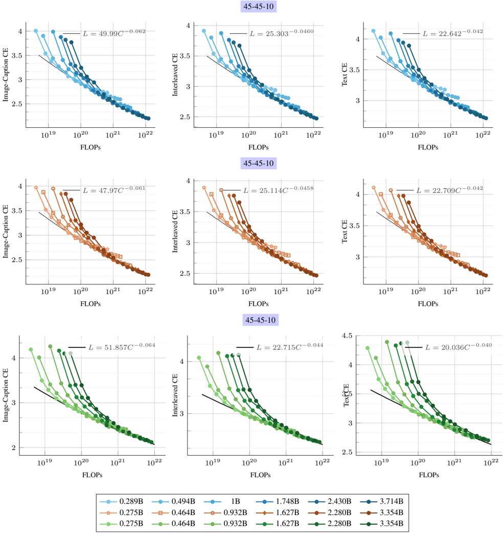
The image contains nine line graphs comparing computational efficiency (CE) metrics across three categories: **Image-Caption CE**, **Interleaved CE**, and **Text CE**. Each graph plots CE against FLOPs (floating-point operations) on a logarithmic scale (10¹⁹ to 10²²). Three datasets are analyzed: **45-45-10**, **45-45-10**, and **45-45-10** (repeated labels suggest a possible typo or repetition in the original image). The graphs use color-coded lines to represent different model sizes (0.275B, 0.464B, 0.932B, 1.627B, 2.280B, 3.354B) and an "IB" baseline. Power-law equations (e.g., *L = a·Cᵇ*) describe the relationship between FLOPs and CE.
---
### Components/Axes
- **X-axis**: FLOPs (logarithmic scale: 10¹⁹ to 10²²)
- **Y-axis**: Computational Efficiency (CE) (linear scale: 2.5 to 4.5)
- **Legends**:
- **Colors**:
- Blue: 0.289B, 0.494B, 1B
- Orange: 0.275B, 0.464B, 0.932B
- Green: 1.627B, 2.280B, 3.354B
- Gray: IB (baseline)
- **Equations**: Power-law relationships (e.g., *L = 49.99C⁻⁰·⁰⁶²*)
---
### Detailed Analysis
#### Image-Caption CE (Top Row)
1. **45-45-10 Dataset**:
- **Blue (0.289B)**: *L = 49.99C⁻⁰·⁰⁶²* (CE decreases slowly with FLOPs).
- **Orange (0.275B)**: *L = 47.97C⁻⁰·⁰⁶¹* (similar trend to 0.289B).
- **Green (1.627B)**: *L = 25.11C⁻⁰·⁰⁴⁸* (steeper decline).
- **Gray (IB)**: *L = 22.64C⁻⁰·⁰⁴²* (lowest CE across FLOPs).
2. **45-45-10 Dataset**:
- **Blue (0.494B)**: *L = 51.85C⁻⁰·⁰⁶⁴* (moderate decline).
- **Orange (0.932B)**: *L = 22.71C⁻⁰·⁰⁴⁴* (steeper than smaller models).
- **Green (2.280B)**: *L = 20.03C⁻⁰·⁰⁴⁰* (most efficient at high FLOPs).
3. **45-45-10 Dataset**:
- **Blue (1B)**: *L = 49.99C⁻⁰·⁰⁶²* (matches 0.289B trend).
- **Orange (2.280B)**: *L = 22.71C⁻⁰·⁰⁴⁴* (consistent with smaller 2.280B).
- **Green (3.354B)**: *L = 20.03C⁻⁰·⁰⁴⁰* (most efficient).
#### Interleaved CE (Middle Row)
- Trends mirror Image-Caption CE, with larger models (e.g., 3.354B) showing steeper declines. For example:
- **3.354B**: *L = 20.03C⁻⁰·⁰⁴⁰* (CE drops sharply with FLOPs).
- **IB**: *L = 22.64C⁻⁰·⁰⁴²* (baseline remains relatively flat).
#### Text CE (Bottom Row)
- Similar patterns: Larger models (e.g., 3.354B) exhibit steeper slopes. For instance:
- **3.354B**: *L = 20.03C⁻⁰·⁰⁴⁰* (CE decreases rapidly).
- **IB**: *L = 22.64C⁻⁰·⁰⁴²* (consistent baseline).
---
### Key Observations
1. **Power-Law Relationships**: All lines follow *L = a·Cᵇ*, where *b* is negative (CE decreases as FLOPs increase).
2. **Model Size Impact**:
- Larger models (e.g., 3.354B) have steeper slopes (*b* closer to -0.04), indicating higher sensitivity to FLOPs.
- Smaller models (e.g., 0.275B) have shallower slopes (*b* closer to -0.06), showing slower CE decline.
3. **IB Baseline**: The "IB" line (gray) consistently shows the lowest CE across all FLOPs, suggesting it represents a less efficient baseline.
4. **Dataset Repetition**: The repeated "45-45-10" labels may indicate a mislabeling or intentional focus on this configuration.
---
### Interpretation
- **Diminishing Returns**: As FLOPs increase, CE improves but at a diminishing rate, consistent with power-law scaling.
- **Model Efficiency**: Larger models achieve higher CE at higher FLOPs but require exponentially more resources to maintain efficiency.
- **Baseline Comparison**: The "IB" line suggests a reference point for evaluating model performance, possibly representing an ideal or standard.
- **Practical Implications**: Optimizing FLOPs is critical for larger models, as their efficiency drops sharply with increased computational load. Smaller models may be more resource-efficient for lower-scale tasks.
---
### Spatial Grounding & Cross-Reference
- **Legend Position**: Bottom of the image, aligned with all graphs.
- **Color Consistency**:
- Blue lines (0.289B, 0.494B, 1B) match across all graphs.
- Orange lines (0.275B, 0.464B, 0.932B) are consistent.
- Green lines (1.627B, 2.280B, 3.354B) align with larger models.
- **Axis Labels**: All graphs share identical axes, ensuring comparability.
---
### Content Details
- **Equations**: Extracted from annotations (e.g., *L = 49.99C⁻⁰·⁰⁶²*).
- **Trends**: All lines slope downward, confirming inverse relationships between FLOPs and CE.
- **Outliers**: No significant outliers; all data points follow expected power-law patterns.
---
### Summary
The graphs demonstrate that computational efficiency (CE) decreases as FLOPs increase, with larger models exhibiting steeper declines. The power-law equations quantify these relationships, highlighting the trade-off between computational resources and efficiency. The "IB" baseline provides a reference for evaluating model performance, while repeated dataset labels suggest a focus on specific configurations.