\n
## Chart: Polynomial Function Plot
### Overview
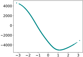
The image displays a plot of a polynomial function. The plot shows a curve that starts at a high positive value, decreases to a negative minimum, and then increases again to a slightly positive value. The x-axis ranges from approximately -3 to 3, and the y-axis ranges from approximately -5000 to 4500. There are a few discrete data points plotted as blue dots along with the continuous curve.
### Components/Axes
* **X-axis:** Labeled with numerical values ranging from -3 to 3, with tick marks at integer values.
* **Y-axis:** Labeled with numerical values ranging from -5000 to 4500, with tick marks at intervals of 1000.
* **Curve:** A teal-colored line representing the polynomial function.
* **Data Points:** Several blue dots are scattered along the curve, indicating specific data points.
### Detailed Analysis
The curve exhibits a cubic-like shape. It begins at approximately x = -3 with a y-value of around 4200. The curve then decreases, crossing the x-axis around x = -1.5. It reaches a minimum value of approximately -4800 at x = 1. The curve then increases, crossing the x-axis again around x = 2.5, and ends at approximately x = 3 with a y-value of around -300.
Here's a breakdown of approximate data points:
* (-3, 4200)
* (-2, 3000)
* (-1, 1000)
* (0, 0)
* (1, -4800)
* (2, -2000)
* (3, -300)
The curve appears smooth and continuous between the plotted data points.
### Key Observations
* The function has at least one local maximum and one local minimum.
* The function crosses the x-axis at least twice, indicating multiple real roots.
* The function is symmetric around the y-axis.
### Interpretation
The plot likely represents a polynomial function of degree 3 or higher. The shape of the curve suggests a cubic function, but higher-degree polynomials could also produce similar shapes. The function's behavior indicates that it has at least two real roots, where the function's value is zero. The symmetry around the y-axis suggests that the function might be an even function, meaning f(x) = f(-x). The data points are likely samples from the continuous function, used to visualize its behavior. The function could be modeling a physical phenomenon where a quantity initially increases, then decreases, and finally increases again, such as the height of a projectile or the temperature change in a system. The exact equation of the polynomial cannot be determined from the plot alone, but it can be approximated using curve fitting techniques.