## Cumulative Distribution Plots: Edges and Heads Sparsity
### Overview
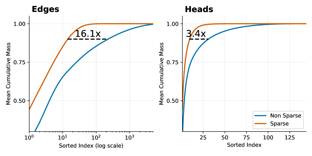
The image presents two cumulative distribution plots, side-by-side. The left plot focuses on "Edges" and the right plot on "Heads". Both plots compare the cumulative mass of "Non Sparse" and "Sparse" data, plotted against a sorted index. The x-axis uses a logarithmic scale for the "Edges" plot. Both plots include a dashed horizontal line indicating a multiplicative factor representing the difference in cumulative mass between the two data types.
### Components/Axes
* **Title (Left):** "Edges" - positioned top-left.
* **Title (Right):** "Heads" - positioned top-left.
* **X-axis (Both):** "Sorted Index" - labeled at the bottom. The "Edges" plot uses a log scale (10^0 to 10^3). The "Heads" plot uses a linear scale (0 to 125).
* **Y-axis (Both):** "Mean Cumulative Mass" - labeled on the left, ranging from 0.0 to 1.0.
* **Legend (Right):** Located in the bottom-right corner.
* "Non Sparse" - represented by a blue line.
* "Sparse" - represented by an orange line.
* **Horizontal Dashed Line (Left):** Labeled "16.1x" - positioned approximately at y=0.95.
* **Horizontal Dashed Line (Right):** Labeled "3.4x" - positioned approximately at y=0.95.
### Detailed Analysis or Content Details
**Edges Plot (Left):**
* **Sparse (Orange):** The orange line representing "Sparse" data exhibits a steep upward slope initially, quickly reaching a cumulative mass of approximately 0.8 by an index of around 10^2 (100). It plateaus around a cumulative mass of 0.95 from an index of approximately 50 to 1000.
* **Non Sparse (Blue):** The blue line representing "Non Sparse" data starts with a gradual slope, increasing more slowly than the "Sparse" data. It reaches a cumulative mass of approximately 0.5 at an index of around 10^1 (10). It continues to increase, but at a slower rate, reaching a cumulative mass of approximately 0.95 at an index of around 10^3 (1000).
* **Difference:** The "Sparse" data reaches a higher cumulative mass for lower sorted indices compared to the "Non Sparse" data. The dashed line indicates that the "Sparse" data achieves a cumulative mass approximately 16.1 times greater than the "Non Sparse" data at the point where the cumulative mass is approximately 0.95.
**Heads Plot (Right):**
* **Sparse (Orange):** The orange line representing "Sparse" data rises rapidly, reaching a cumulative mass of approximately 0.75 by an index of 25. It plateaus around a cumulative mass of 0.95 from an index of approximately 50.
* **Non Sparse (Blue):** The blue line representing "Non Sparse" data starts with a slower slope, gradually increasing. It reaches a cumulative mass of approximately 0.5 at an index of around 25. It continues to increase, approaching a cumulative mass of 0.95 at an index of around 100.
* **Difference:** Similar to the "Edges" plot, the "Sparse" data reaches a higher cumulative mass for lower sorted indices. The dashed line indicates that the "Sparse" data achieves a cumulative mass approximately 3.4 times greater than the "Non Sparse" data at the point where the cumulative mass is approximately 0.95.
### Key Observations
* In both plots, the "Sparse" data consistently exhibits a higher cumulative mass for lower sorted indices compared to the "Non Sparse" data.
* The difference in cumulative mass between "Sparse" and "Non Sparse" data is more pronounced in the "Edges" plot (16.1x) than in the "Heads" plot (3.4x).
* The "Edges" plot uses a logarithmic scale on the x-axis, which compresses the distribution of indices.
### Interpretation
These plots demonstrate the impact of sparsity on the cumulative mass of "Edges" and "Heads" features. The higher cumulative mass of "Sparse" data at lower indices suggests that a significant portion of the total mass is concentrated in a smaller number of features when sparsity is applied. The larger multiplicative factor for "Edges" (16.1x) indicates that sparsity has a more substantial effect on the distribution of "Edges" features compared to "Heads" features. This could imply that "Edges" are more amenable to sparsity-inducing techniques or that the underlying data distribution of "Edges" naturally lends itself to sparsity. The plots suggest that applying sparsity can effectively capture the most important features (those contributing to the initial cumulative mass) while potentially discarding less relevant ones. The difference in the multiplicative factors between "Edges" and "Heads" suggests that the effectiveness of sparsity may vary depending on the type of feature being considered.